Quickstart
In this Quickstart, we’ll train a semantic segmentation model on SpaceNet data. Don’t get too excited - we’ll only be training for a very short time on a very small training set! So the model that is created here will be pretty much worthless. But! These steps will show how Raster Vision pipelines are set up and run, so when you are ready to run against a lot of training data for a longer time on a GPU, you’ll know what you have to do. Also, we’ll show how to make predictions on the data using a model we’ve already trained on GPUs to show what you can expect to get out of Raster Vision.
For the Quickstart we are going to be using one of the published Docker Images as it has an environment with all necessary dependencies already installed.
See also
It is also possible to install Raster Vision using pip, but it can be time-consuming and error-prone to install all the necessary dependencies. See Installing via pip for more details.
Note
This Quickstart requires a Docker installation. We have tested this with Docker 19, although you may be able to use a lower version. See Get Started with Docker for installation instructions.
You’ll need to choose two directories, one for keeping your configuration source file and another for holding experiment output. Make sure these directories exist:
> export RV_QUICKSTART_CODE_DIR=`pwd`/code
> export RV_QUICKSTART_OUT_DIR=`pwd`/output
> mkdir -p ${RV_QUICKSTART_CODE_DIR} ${RV_QUICKSTART_OUT_DIR}
Now we can run a console in the the Docker container by doing
> docker run --rm -it \
     -v ${RV_QUICKSTART_CODE_DIR}:/opt/src/code  \
     -v ${RV_QUICKSTART_OUT_DIR}:/opt/data/output \
     quay.io/azavea/raster-vision:pytorch-0.12 /bin/bash
See also
See Docker Images for more information about setting up Raster Vision with Docker images.
The Data
Configuring a semantic segmentation pipeline
Create a Python file in the ${RV_QUICKSTART_CODE_DIR} named tiny_spacenet.py. Inside, you’re going to write a function called get_config that returns a SemanticSegmentationConfig object. This object’s type is a subclass of PipelineConfig, and configures a semantic segmentation pipeline which analyzes the imagery, creates training chips, trains a model, makes predictions on validation scenes, evaluates the predictions, and saves a model bundle.
# flake8: noqa

from os.path import join

from rastervision.core.rv_pipeline import *
from rastervision.core.backend import *
from rastervision.core.data import *
from rastervision.pytorch_backend import *
from rastervision.pytorch_learner import *


def get_config(runner):
    root_uri = '/opt/data/output/'
    base_uri = ('https://s3.amazonaws.com/azavea-research-public-data/'
                'raster-vision/examples/spacenet')
    train_image_uri = '{}/RGB-PanSharpen_AOI_2_Vegas_img205.tif'.format(
        base_uri)
    train_label_uri = '{}/buildings_AOI_2_Vegas_img205.geojson'.format(
        base_uri)
    val_image_uri = '{}/RGB-PanSharpen_AOI_2_Vegas_img25.tif'.format(base_uri)
    val_label_uri = '{}/buildings_AOI_2_Vegas_img25.geojson'.format(base_uri)
    channel_order = [0, 1, 2]
    class_config = ClassConfig(
        names=['building', 'background'], colors=['red', 'black'])

    def make_scene(scene_id, image_uri, label_uri):
        """
        - StatsTransformer is used to convert uint16 values to uint8.
        - The GeoJSON does not have a class_id property for each geom,
          so it is inferred as 0 (ie. building) because the default_class_id
          is set to 0.
        - The labels are in the form of GeoJSON which needs to be rasterized
          to use as label for semantic segmentation, so we use a RasterizedSource.
        - The rasterizer set the background (as opposed to foreground) pixels
          to 1 because background_class_id is set to 1.
        """
        raster_source = RasterioSourceConfig(
            uris=[image_uri],
            channel_order=channel_order,
            transformers=[StatsTransformerConfig()])
        vector_source = GeoJSONVectorSourceConfig(
            uri=label_uri, default_class_id=0, ignore_crs_field=True)
        label_source = SemanticSegmentationLabelSourceConfig(
            raster_source=RasterizedSourceConfig(
                vector_source=vector_source,
                rasterizer_config=RasterizerConfig(background_class_id=1)))
        return SceneConfig(
            id=scene_id,
            raster_source=raster_source,
            label_source=label_source)

    dataset = DatasetConfig(
        class_config=class_config,
        train_scenes=[
            make_scene('scene_205', train_image_uri, train_label_uri)
        ],
        validation_scenes=[
            make_scene('scene_25', val_image_uri, val_label_uri)
        ])

    # Use the PyTorch backend for the SemanticSegmentation pipeline.
    chip_sz = 300
    backend = PyTorchSemanticSegmentationConfig(
        model=SemanticSegmentationModelConfig(backbone=Backbone.resnet50),
        solver=SolverConfig(lr=1e-4, num_epochs=1, batch_sz=2))
    chip_options = SemanticSegmentationChipOptions(
        window_method=SemanticSegmentationWindowMethod.random_sample,
        chips_per_scene=10)

    return SemanticSegmentationConfig(
        root_uri=root_uri,
        dataset=dataset,
        backend=backend,
        train_chip_sz=chip_sz,
        predict_chip_sz=chip_sz,
        chip_options=chip_options)
Running the pipeline
We can now run the pipeline by invoking the following command inside the container.
> rastervision run local code/tiny_spacenet.py
Seeing Results
If you go to ${RV_QUICKSTART_OUT_DIR} you should see a directory structure like this.
Note
This uses the tree command which you may need to install first.
> tree -L 3
 .
 ├── analyze
 │   └── stats.json
 ├── bundle
 │   └── model-bundle.zip
 ├── chip
 │   └── 3113ff8c-5c49-4d3c-8ca3-44d412968108.zip
 ├── eval
 │   └── eval.json
 ├── pipeline-config.json
 ├── predict
 │   └── scene_25.tif
 └── train
     ├── dataloaders
     │   ├── test.png
     │   ├── train.png
     │   └── valid.png
     ├── last-model.pth
     ├── learner-config.json
     ├── log.csv
     ├── model-bundle.zip
     ├── tb-logs
     │   └── events.out.tfevents.1585513048.086fdd4c5530.214.0
     ├── test_metrics.json
     └── test_preds.png
The root directory contains a serialized JSON version of the configuration at pipeline-config.json, and each subdirectory with a command name contains output for that command. You can see test predictions on a batch of data in train/test_preds.png, and evaluation metrics in eval/eval.json, but don’t get too excited! We
trained a model for 1 epoch on a tiny dataset, and the model is likely making random predictions at this point. We would need to
train on a lot more data for a lot longer for the model to become good at this task.
Model Bundles
To immediately use Raster Vision with a fully trained model, one can make use of the pretrained models in our Model Zoo. However, be warned that these models probably won’t work well on imagery taken in a different city, with a different ground sampling distance, or different sensor.
For example, to use a DeepLab/Resnet50 model that has been trained to do building segmentation on Las Vegas, one can type:
> rastervision predict https://s3.amazonaws.com/azavea-research-public-data/raster-vision/examples/model-zoo-0.12/spacenet-vegas-buildings-ss/model-bundle.zip https://s3.amazonaws.com/azavea-research-public-data/raster-vision/examples/model-zoo-0.12/spacenet-vegas-buildings-ss/1929.tif prediction.tif
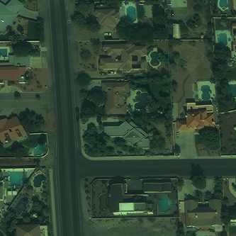
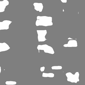
This will make predictions on the image 1929.tif using the provided model bundle, and will produce a file called predictions.tif. These files are in GeoTiff format, and you will need a GIS viewer such as QGIS to open them correctly on your device. Notice that the prediction package and the input raster are transparently downloaded via HTTP.
The input image (false color) and predictions are reproduced below.
See also
You can read more about the model bundle concept and the predict CLI command in the documentation.