Note

This page was generated from pred_and_eval_ss.ipynb.

Note

If running outside of the Docker image, you might need to set a couple of environment variables manually. You can do it like so:

import os
from subprocess import check_output

os.environ['GDAL_DATA'] = check_output('pip show rasterio | grep Location | awk \'{print $NF"/rasterio/gdal_data/"}\'', shell=True).decode().strip()
os.environ['AWS_NO_SIGN_REQUEST'] = 'YES'

See this Colab notebook for an example.

Prediction and Evaluation#

Load a `Learner` with a trained model from bundle – `Learner.from_model_bundle()`#

[1]:

bundle_uri = 'https://s3.amazonaws.com/azavea-research-public-data/raster-vision/examples/model-zoo-0.20/spacenet-vegas-buildings-ss/train/model-bundle.zip'

[2]:

from rastervision.pytorch_learner import SemanticSegmentationLearner

learner = SemanticSegmentationLearner.from_model_bundle(bundle_uri, training=False)

2022-11-09 13:01:57:rastervision.pytorch_learner.learner: INFO - Loading learner from bundle https://s3.amazonaws.com/azavea-research-public-data/raster-vision/examples/model-zoo-0.13/spacenet-vegas-buildings-ss/train/model-bundle.zip.
2022-11-09 13:01:57:rastervision.pipeline.file_system.utils: INFO - Using cached file /opt/data/tmp/cache/http/s3.amazonaws.com/azavea-research-public-data/raster-vision/examples/model-zoo-0.13/spacenet-vegas-buildings-ss/train/model-bundle.zip.
2022-11-09 13:02:03:rastervision.pytorch_learner.learner: INFO - Local output dir: /opt/data/tmp/tmpyt368dek/s3/raster-vision/examples/0.13/output/spacenet-vegas-buildings-ss/train
2022-11-09 13:02:03:rastervision.pytorch_learner.learner: INFO - Remote output dir: s3://raster-vision/examples/0.13/output/spacenet-vegas-buildings-ss/train
2022-11-09 13:02:06:rastervision.pytorch_learner.learner: INFO - Loading model weights from: /opt/data/tmp/tmpyt368dek/model-bundle/model.pth

Note

If you used a custom model instead of using ModelConfig while training, you will need to initialize that model again and pass it to Learner.from_model_bundle(). See the Training a model tutorial for an example.

Get scene to predict#

[3]:

scene_id = 5631
image_uri = f's3://spacenet-dataset/spacenet/SN2_buildings/train/AOI_2_Vegas/PS-RGB/SN2_buildings_train_AOI_2_Vegas_PS-RGB_img{scene_id}.tif'
label_uri = f's3://spacenet-dataset/spacenet/SN2_buildings/train/AOI_2_Vegas/geojson_buildings/SN2_buildings_train_AOI_2_Vegas_geojson_buildings_img{scene_id}.geojson'

[4]:

from rastervision.core.data import ClassConfig

class_config = ClassConfig(
    names=['building', 'background'],
    colors=['orange', 'black'])
class_config.ensure_null_class()

[5]:

from rastervision.core.data import ClassConfig
from rastervision.pytorch_learner import SemanticSegmentationSlidingWindowGeoDataset

import albumentations as A

ds = SemanticSegmentationSlidingWindowGeoDataset.from_uris(
    class_config=class_config,
    image_uri=image_uri,
    size=325,
    stride=325,
    transform=A.Resize(325, 325))

2022-11-09 13:02:35:rastervision.pipeline.file_system.utils: INFO - Using cached file /opt/data/tmp/cache/s3/spacenet-dataset/spacenet/SN2_buildings/train/AOI_2_Vegas/PS-RGB/SN2_buildings_train_AOI_2_Vegas_PS-RGB_img5631.tif.
2022-11-09 13:02:36:rastervision.core.data.raster_source.rasterio_source: WARNING - Raster block size (2, 650) is too non-square. This can slow down reading. Consider re-tiling using GDAL.

Predict – `Learner.predict_dataset()`#

Make predictions via Learner.predict_dataset() and then turn them into Labels via Labels.from_predictions (specifically, SemanticSegmentationLabels.from_predictions).

[6]:

from rastervision.core.data import SemanticSegmentationLabels

predictions = learner.predict_dataset(
    ds,
    raw_out=True,
    numpy_out=True,
    predict_kw=dict(out_shape=(325, 325)),
    progress_bar=True)

pred_labels = SemanticSegmentationLabels.from_predictions(
    ds.windows,
    predictions,
    smooth=True,
    extent=ds.scene.extent,
    num_classes=len(class_config))

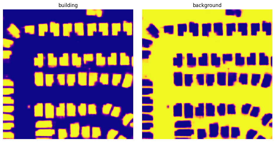
Visualize predictions#

pred_labels is an instance of SemanticSegmentationSmoothLabels which is a raster of probability distributions for each pixel for the entire scene. We can get these probabilities via get_score_arr().

Note

There is also a get_label_arr() method that will return a 2D raster of class IDs representing the most probable class for each pixel.

[7]:

scores = pred_labels.get_score_arr(pred_labels.extent)

[8]:

from matplotlib import pyplot as plt

scores_building = scores[0]
scores_background = scores[1]

fig, (ax1, ax2) = plt.subplots(1, 2, figsize=(10, 5))
fig.tight_layout(w_pad=-2)
ax1.imshow(scores_building, cmap='plasma')
ax1.axis('off')
ax1.set_title('building')
ax2.imshow(scores_background, cmap='plasma')
ax2.axis('off')
ax2.set_title('background')
plt.show()

../../_images/usage_tutorials_pred_and_eval_ss_18_0.png

Save predictions to file – `SemanticSegmentationSmoothLabels.save()`#

[7]:

pred_labels.save(
    uri=f'./spacenet-vegas-buildings-ss/predict/{scene_id}',
    crs_transformer=ds.scene.raster_source.crs_transformer,
    class_config=class_config)

Evaluate predictions#

We now want to evaluate the predictions against the ground truth labels.

Raster Vision allows us to do this via an Evaluator. In our case, this would be the SemanticSegmentationEvaluator. We are going to use its evaluate_predictions() method, which takes both ground truth labels and predictions as Labels objects.

We already have the predictions as a SemanticSegmentationLabels object, so we just need to load the ground truth labels as SemanticSegmentationLabels too. We do that by using make_ss_scene() factory function to create a scene and then accessing scene.label_source.get_labels(). Alternatively, we could have directly created a SemanticSegmentationLabelSource.

[10]:

from rastervision.core.data.utils import make_ss_scene

scene = make_ss_scene(
    class_config=class_config,
    image_uri=image_uri,
    label_vector_uri=label_uri,
    label_vector_default_class_id=class_config.get_class_id('building'),
    label_raster_source_kw=dict(
        background_class_id=class_config.get_class_id('background')),
    image_raster_source_kw=dict(allow_streaming=True))

gt_labels = scene.label_source.get_labels()

2022-10-21 10:06:26:rastervision.pipeline.file_system.utils: INFO - Using cached file /opt/data/tmp/cache/s3/spacenet-dataset/spacenet/SN2_buildings/train/AOI_2_Vegas/geojson_buildings/SN2_buildings_train_AOI_2_Vegas_geojson_buildings_img5631.geojson.

Note

gt_labels is an instance of SemanticSegmentationDiscreteLabels. You can convert it to a label raster (for visualization or some other analysis) via get_label_arr().

[11]:

from rastervision.core.evaluation import SemanticSegmentationEvaluator

evaluator = SemanticSegmentationEvaluator(class_config)

evaluation = evaluator.evaluate_predictions(
    ground_truth=gt_labels, predictions=pred_labels)

SemanticSegmentationEvaluator.evaluate_predictions() returns a SemanticSegmentationEvaluation object which contains evaluations for each class as ClassEvaluationItem objects.

We can examine these evaluations as shown below.

Evaluation for the building class:

[12]:

evaluation.class_to_eval_item[0]

[12]:

{'class_id': 0,
 'class_name': 'building',
 'conf_mat': [[289042.0, 12212.0], [9351.0, 111895.0]],
 'conf_mat_dict': {'FN': 9351.0, 'FP': 12212.0, 'TN': 289042.0, 'TP': 111895.0},
 'conf_mat_frac': [[0.684123076923077, 0.02890414201183432],
                   [0.022132544378698226, 0.2648402366863905]],
 'conf_mat_frac_dict': {'FN': 0.022132544378698226,
                        'FP': 0.02890414201183432,
                        'TN': 0.684123076923077,
                        'TP': 0.2648402366863905},
 'count_error': 2861.0,
 'gt_count': 121246.0,
 'metrics': {'f1': 0.9121143821351279,
             'precision': 0.9016010378141442,
             'recall': 0.9228758062121637,
             'sensitivity': 0.9228758062121637,
             'specificity': 0.9594627789174583},
 'pred_count': 124107.0,
 'relative_frequency': 0.2869727810650888}

Evaluation for the background class:

[13]:

evaluation.class_to_eval_item[1]

[13]:

{'class_id': 1,
 'class_name': 'background',
 'conf_mat': [[111895.0, 9351.0], [12212.0, 289042.0]],
 'conf_mat_dict': {'FN': 12212.0, 'FP': 9351.0, 'TN': 111895.0, 'TP': 289042.0},
 'conf_mat_frac': [[0.2648402366863905, 0.022132544378698226],
                   [0.02890414201183432, 0.684123076923077]],
 'conf_mat_frac_dict': {'FN': 0.02890414201183432,
                        'FP': 0.022132544378698226,
                        'TN': 0.2648402366863905,
                        'TP': 0.684123076923077},
 'count_error': 2861.0,
 'gt_count': 301254.0,
 'metrics': {'f1': 0.9640405105003443,
             'precision': 0.9686621334950887,
             'recall': 0.9594627789174583,
             'sensitivity': 0.9594627789174583,
             'specificity': 0.9228758062121637},
 'pred_count': 298393.0,
 'relative_frequency': 0.7130272189349113}

Save evaluation#

We can also save the evaluations as a JSON via SemanticSegmentationEvaluation.save()

[14]:

evaluation.save(f'eval-{scene_id}.json')

Prediction and Evaluation#

Load a Learner with a trained model from bundle – Learner.from_model_bundle()#

Get scene to predict#

Predict – Learner.predict_dataset()#

Visualize predictions#

Save predictions to file – SemanticSegmentationSmoothLabels.save()#

Evaluate predictions#

Save evaluation#

Load a `Learner` with a trained model from bundle – `Learner.from_model_bundle()`#

Predict – `Learner.predict_dataset()`#

Save predictions to file – `SemanticSegmentationSmoothLabels.save()`#