Note
This page was generated from stac_plus_osm.ipynb.
Note
If running outside of the Docker image, you may need to set some environment variables manually. You can do it like so:
import os
from subprocess import check_output

os.environ['GDAL_DATA'] = check_output('pip show rasterio | grep Location | awk \'{print $NF"/rasterio/gdal_data/"}\'', shell=True).decode().strip()
Imagery from STAC API + labels from OSM#
This notebook demonstrates a workflow where Sentinel-2 imagery from a STAC API is combined with annotations from OpenStreetMap to create a GeoDataset that can be used to train a model.
For this example, our labels will be OSM labels for roads, our AOI will be the city of Paris, France, and the STAC API we will use is Earth Search.
Install dependencies#
[ ]:
%pip install osm2geojson==0.2.4 pystac_client==0.6.1 stackstac==0.4.4
[ ]:
from rastervision.pipeline.file_system.utils import json_to_file
from rastervision.core.box import Box
from rastervision.core.data import (RasterioCRSTransformer, StatsTransformer,
                                    XarraySource)
from rastervision.core.data.raster_source import XarraySource
from rastervision.core.data.utils import (geoms_to_geojson, geojson_to_geoms,
                                          get_polygons_from_uris)

from shapely.geometry import mapping
from matplotlib import pyplot as plt
import seaborn as sns
sns.reset_defaults()
Get labels from OSM via overpass API#
[3]:
import requests
import osm2geojson
from shapely.ops import unary_union

overpass_api_endpoint = 'https://overpass-api.de/api/interpreter'


def fetch_osm_geojson(query: str) -> dict:
    response = requests.get(
        f'{overpass_api_endpoint}?data=[out:xml][timeout:25];{query};out geom;'
    )
    string = response.text.replace("\n", "")
    geojson = osm2geojson.xml2geojson(string)
    return geojson


def get_city_boundary(country: str, city: str) -> Box:
    query = f"""
    area[name="{country}"][admin_level=2]->.country;
    area[name="{city}"][boundary=administrative](area.country);
    (
        way(area.country)[name="{city}"][boundary=administrative];
        relation(area.country)[name="{city}"][boundary=administrative];
    )
    """
    geojson = fetch_osm_geojson(query)
    geom = unary_union(list(geojson_to_geoms(geojson)))
    return geom


def get_city_bbox(country: str, city: str) -> Box:
    geom = get_city_boundary(country, city)
    city_bbox = Box.from_shapely(geom.envelope)
    return city_bbox


def get_city_features(country: str, city: str, query: str) -> dict:
    query_city = f"""
    area[name="{country}"][admin_level=2]->.country;
    area[name="{city}"][boundary=administrative](area.country)->.city;
    ({query})
    """
    geojson = fetch_osm_geojson(query_city)
    return geojson
We’ll use road labels for Paris, France. In OSM, the super-category for all kinds of roads is “highway”.
[4]:
country = 'France'
city = 'Paris'
query_road = f'way(area.country)(area.city)["highway"];'

filename_features = f'roads_{city}.json'
filename_aoi = f'aoi_{city}.json'
[5]:
geojson = get_city_features(country, city, query_road)
print(f'Features found: {len(geojson["features"])}')

print(f'Saving to {filename_features}')
json_to_file(geojson, filename_features)

aoi = get_city_boundary(country, city)
aoi_geojson = geoms_to_geojson([aoi])
print(f'Saving AOI to {filename_aoi}')
json_to_file(aoi_geojson, filename_aoi)
Features found: 92442
Saving to roads_Paris.json
Saving AOI to aoi_Paris.json
Get Sentinel-2 imagery from STAC API as a DataArray#
[5]:
import pystac_client
import stackstac
We’ll query the STAC API for items that intersect with the city’s bounding box.
[6]:
# get city bounding box from OSM
bbox = get_city_bbox(country, city)
bbox_geometry = mapping(bbox.to_shapely())
bbox, bbox_geometry
[6]:
(Box(ymin=48.8155755, xmin=2.224122, ymax=48.902156, xmax=2.4697602),
 {'type': 'Polygon',
  'coordinates': (((2.224122, 48.8155755),
    (2.224122, 48.902156),
    (2.4697602, 48.902156),
    (2.4697602, 48.8155755),
    (2.224122, 48.8155755)),)})
Get items from the “Sentinel-2 L2A COGs” collection between 15 March 2023 and 7 April 2023, that intersect with the city’s bounding box.
[12]:
URL = "https://earth-search.aws.element84.com/v1"
catalog = pystac_client.Client.open(URL)

items = catalog.search(
    intersects=bbox_geometry,
    collections=["sentinel-2-l2a"],
    datetime="2023-03-15/2023-04-07",
    query={"eo:cloud_cover": {"lt": 5}},
).get_all_items()

stack = stackstac.stack(items)
stack
[12]:
<xarray.DataArray 'stackstac-c221d8123b0a1e61acf10801cf3e5756' (time: 1,
                                                                band: 32,
                                                                y: 10980,
                                                                x: 10980)>
dask.array<fetch_raster_window, shape=(1, 32, 10980, 10980), dtype=float64, chunksize=(1, 1, 1024, 1024), chunktype=numpy.ndarray>
Coordinates: (12/52)
  * time                                     (time) datetime64[ns] 2023-04-03...
    id                                       (time) <U24 'S2B_31UDQ_20230403_...
  * band                                     (band) <U12 'aot' ... 'wvp-jp2'
  * x                                        (x) float64 4e+05 ... 5.098e+05
  * y                                        (y) float64 5.5e+06 ... 5.39e+06
    view:sun_azimuth                         float64 163.6
    ...                                       ...
    raster:bands                             (band) object [{'nodata': 0, 'da...
    gsd                                      (band) object None 10 ... None None
    common_name                              (band) object None 'blue' ... None
    center_wavelength                        (band) object None 0.49 ... None
    full_width_half_max                      (band) object None 0.098 ... None
    epsg                                     int64 32631
Attributes:
    spec:        RasterSpec(epsg=32631, bounds=(399960.0, 5390220.0, 509760.0...
    crs:         epsg:32631
    transform:   | 10.00, 0.00, 399960.00|\n| 0.00,-10.00, 5500020.00|\n| 0.0...
resolution: 10.0Convert to a Raster Vision RasterSource#
We need a CRSTransformer to ensure correct alignment of georeferenced imagery and labels.
[8]:
crs_transformer = RasterioCRSTransformer(
    transform=stack.transform, image_crs=stack.crs)
Subset the DataArray to a single timestamp and the 12 Sentinel-2 L2A bands.
[9]:
data_array = stack
data_array = data_array.isel(time=-1)
data_array = data_array.sel(
    band=[
        'coastal', # B01
        'blue', # B02
        'green', # B03
        'red', # B04
        'rededge1', # B05
        'rededge2', # B06
        'rededge3', # B07
        'nir', # B08
        'nir08', # B8A
        'nir09', # B09
        'swir16', # B11
        'swir22', # B12
    ])
Create a RasterSource (specifically, an XarraySource) from the DataArray. Also, use StatsTransformer to normalize the pixels values.
Note that XarraySource is agnostic to the DataArray backend. Which means you can also pass it a DataArray backed by a Dask cluster.
[10]:
bbox_pixel_coords = crs_transformer.map_to_pixel(bbox).normalize()

raster_source_unnormalized = XarraySource(
    data_array,
    crs_transformer=crs_transformer,
    bbox=bbox_pixel_coords,
)
stats_tf = StatsTransformer.from_raster_sources([raster_source_unnormalized])

raster_source = XarraySource(
    data_array,
    crs_transformer=crs_transformer,
    raster_transformers=[stats_tf],
    bbox=bbox_pixel_coords,
)
raster_source.shape
[10]:
(947, 1810, 12)
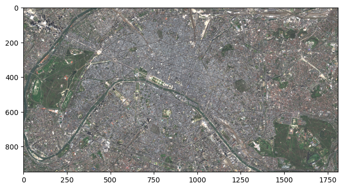
Visualize the full image (within the city’s bounding box):
[13]:
chip = raster_source[:, :, [3, 2, 1]]
chip.shape

fig, ax = plt.subplots(1, 1, figsize=(8, 8))
ax.imshow(chip)
plt.show()
Read in the OSM labels as a LabelSource#
[14]:
from rastervision.core.data import (ClassConfig, GeoJSONVectorSource,
                                    RasterizedSource, Scene,
                                    SemanticSegmentationLabelSource)
from rastervision.core.data.vector_transformer import (
    BufferTransformer, ClassInferenceTransformer)
from rastervision.pytorch_learner import (
    SemanticSegmentationRandomWindowGeoDataset,
    SemanticSegmentationSlidingWindowGeoDataset,
    SemanticSegmentationVisualizer)

labels_uri = filename_features

class_config = ClassConfig(
    names=['background', 'road'],
    colors=['lightgray', 'black'],
    null_class='background')
Note how below we use ClassInferenceTransformer to assign classes to features. Here, class_id_to_filter is redundant given we’re using default_class_id=road_class_id (which means all features will be assigned that class ID), but if we, for example, wanted to restrict to certain types of road, or to have different classes for each type of roads, class_id_to_filter would allow us to do that.
[15]:
road_class_id = class_config.get_class_id('road')

label_vector_source = GeoJSONVectorSource(
    labels_uri,
    crs_transformer=crs_transformer,
    ignore_crs_field=True,
    vector_transformers=[
        # assign class IDs to features in the GeoJSON
        ClassInferenceTransformer(
            # Here, this is redundant given we're using default_class_id=road_class_id,
            # but if we, for example, wanted to restrict to certain types of road,
            # or to have different classes from each type of road, we could do that
            # using class_id_to_filter.
            class_id_to_filter={
                road_class_id: ['in', 'tags', 'highway'],
            },
            default_class_id=road_class_id),
        # OSM represents roads as LineStrings, buffer them into polygons
        BufferTransformer('LineString', class_bufs={1: 0.5}),
    ])
label_raster_source = RasterizedSource(
    label_vector_source,
    background_class_id=class_config.null_class_id,
    all_touched=True,
)
label_source = SemanticSegmentationLabelSource(label_raster_source,
                                               class_config)
2023-07-20 19:33:24:rastervision.core.data.vector_source.vector_source: WARNING - Invalid geometries found in features in the GeoJSON.
Create a GeoDataset for the scene#
Specifically, a SemanticSegmentationRandomWindowGeoDataset.
[16]:
aoi_polygons = get_polygons_from_uris(filename_aoi, crs_transformer)
scene = Scene(
    id='test_scene',
    raster_source=raster_source,
    label_source=label_source,
    aoi_polygons=aoi_polygons,
)
ds = SemanticSegmentationRandomWindowGeoDataset(
    scene=scene, size_lims=(200, 201), out_size=256)
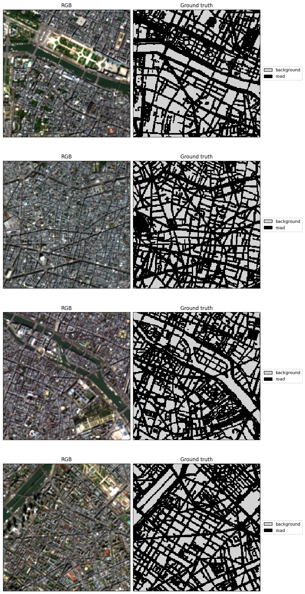
Visualize sample chips from the dataset#
[17]:
viz = SemanticSegmentationVisualizer(
    class_names=class_config.names,
    class_colors=class_config.colors,
    channel_display_groups=dict(RGB=[3, 2, 1]))
viz.scale = 5
[18]:
x, y = viz.get_batch(ds, 4)
viz.plot_batch(x, y, show=True)
What next?#
Take a look at the training tutorial to see how you can use this dataset for training!