Note
This page was generated from temporal.ipynb.
Note
If running outside of the Docker image, you may need to set some environment variables manually. You can do it like so:
import os
from subprocess import check_output

os.environ['GDAL_DATA'] = check_output('pip show rasterio | grep Location | awk \'{print $NF"/rasterio/gdal_data/"}\'', shell=True).decode().strip()
Working with time-series of images#
This notebook demonstrates how you can use time-series data with Raster Vision. We will query a STAC API for a spatiotemporal data cube and use a temporal model to run inference on it.
In particular, we will use a simple pre-trained model that computes attention scores for each image in the time-series. We will see that images with cloud cover get assigned lower attention scores.
Install dependencies#
[ ]:
%pip install pystac_client==0.6.1 stackstac==0.4.4
[ ]:
from rastervision.core.box import Box
from rastervision.core.data import (RasterioCRSTransformer, StatsTransformer,
                                    XarraySource)
from rastervision.core.data.raster_source import XarraySource

from rastervision.core.data import Scene
from rastervision.pytorch_learner import (
    SemanticSegmentationRandomWindowGeoDataset)

import math
import torch
from shapely.geometry import mapping
from matplotlib import pyplot as plt
import seaborn as sns
sns.reset_defaults()

DEVICE = 'cuda' if torch.cuda.is_available() else 'cpu'
Get a time-series of Sentinel-2 images from a STAC API#
Get Sentinel-2 imagery from 2023-06-01 to 2023-06-20 over Paris, France.
[3]:
import pystac_client
import stackstac
[4]:
bbox = Box(ymin=48.8155755, xmin=2.224122, ymax=48.902156, xmax=2.4697602)
bbox_geometry = mapping(bbox.to_shapely().oriented_envelope)
[5]:
URL = "https://earth-search.aws.element84.com/v1"
catalog = pystac_client.Client.open(URL)

items = catalog.search(
    intersects=bbox_geometry,
    collections=["sentinel-2-l2a"],
    datetime="2023-06-01/2023-06-20",
).get_all_items()

stack = stackstac.stack(items)
stack
[5]:
<xarray.DataArray 'stackstac-324721a98d3cff22ae730b7f1736dac4' (time: 6,
                                                                band: 32,
                                                                y: 10980,
                                                                x: 10980)>
dask.array<fetch_raster_window, shape=(6, 32, 10980, 10980), dtype=float64, chunksize=(1, 1, 1024, 1024), chunktype=numpy.ndarray>
Coordinates: (12/52)
  * time                                     (time) datetime64[ns] 2023-06-02...
    id                                       (time) <U24 'S2B_31UDQ_20230602_...
  * band                                     (band) <U12 'aot' ... 'wvp-jp2'
  * x                                        (x) float64 4e+05 ... 5.098e+05
  * y                                        (y) float64 5.5e+06 ... 5.39e+06
    mgrs:grid_square                         <U2 'DQ'
    ...                                       ...
    raster:bands                             (band) object [{'nodata': 0, 'da...
    gsd                                      (band) object None 10 ... None None
    common_name                              (band) object None 'blue' ... None
    center_wavelength                        (band) object None 0.49 ... None
    full_width_half_max                      (band) object None 0.098 ... None
    epsg                                     int64 32631
Attributes:
    spec:        RasterSpec(epsg=32631, bounds=(399960.0, 5390220.0, 509760.0...
    crs:         epsg:32631
    transform:   | 10.00, 0.00, 399960.00|\n| 0.00,-10.00, 5500020.00|\n| 0.0...
resolution: 10.0Convert to a Raster Vision RasterSource#
We need a CRSTransformer to ensure we can correctly geospatially align this imagery with other imagery or with labels.
[6]:
crs_transformer = RasterioCRSTransformer(
    transform=stack.transform, image_crs=stack.crs)
Subset the DataArray to the 12 Sentinel-2 L2A bands in the order that the model expects.
[7]:
data_array = stack
data_array = data_array.sel(
    band=[
        'coastal', # B01
        'blue', # B02
        'green', # B03
        'red', # B04
        'rededge1', # B05
        'rededge2', # B06
        'rededge3', # B07
        'nir', # B08
        'nir08', # B8A
        'nir09', # B09
        'swir16', # B11
        'swir22', # B12
    ])
Create the RasterSource#
[22]:
bbox_pixel_coords = crs_transformer.map_to_pixel(bbox).normalize()

raster_source_unnormalized = XarraySource(
    data_array,
    crs_transformer=crs_transformer,
    bbox=bbox_pixel_coords,
    temporal=True)
raster_source_unnormalized.shape
[22]:
(6, 947, 1810, 12)
The model expects unnormalized data, but we do need to normalize it if we want to visualize it. Below, we compute stats from the first 2 images in the sequence since they are free of clouds (this was determined by inspecting the images). We then use those stats to create a normalized version of the same RasterSource as above but with only the red, green, and blue bands.
[18]:
raster_source_stats = XarraySource(
    data_array.isel(time=[0, 1]),
    crs_transformer=crs_transformer,
    bbox=bbox_pixel_coords,
    temporal=True)

stats_tf = StatsTransformer.from_raster_sources([raster_source_stats])

raster_source_viz = XarraySource(
    data_array,
    channel_order=[3, 2, 1],  # RGB
    crs_transformer=crs_transformer,
    raster_transformers=[stats_tf],
    bbox=bbox_pixel_coords,
    temporal=True)
raster_source_viz.shape
[18]:
(6, 947, 1810, 3)
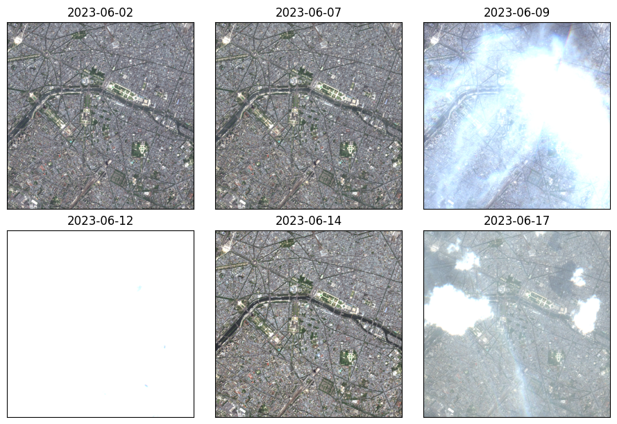
Visualize the images in the time-series:
[13]:
T = raster_source_viz.shape[0]
t_strs = [str(s.date()) for s in raster_source_viz.data_array.time.to_series()]

ncols = 3
nrows = int(math.ceil(T / ncols))
fig, axs = plt.subplots(
    nrows, ncols, figsize=(ncols * 3, nrows * 3), constrained_layout=True)
for t, t_str, ax in zip(range(T), t_strs, axs.flat):
    chip = raster_source_viz[t, 200:800, 400:1000]
    ax.imshow(chip)
    ax.set_title(t_str, fontsize=12)
    ax.tick_params(top=False, bottom=False, left=False, right=False,
                labelleft=False, labelbottom=False, labeltop=False)
plt.show()
Get model#
We will use a model from a fork of https://github.com/jamesmcclain/geospatial-time-series.
[10]:
model_weights_path = 'https://s3.amazonaws.com/azavea-research-public-data/raster-vision/examples/tutorials-data/temporal/pretrained-resnet18-weights.pth'
[ ]:
model = torch.hub.load(
    'AdeelH/geospatial-time-series:rv-demo',
    'SeriesResNet18',
    source='github',
    trust_repo=False,
)
model.load_state_dict(torch.hub.load_state_dict_from_url(model_weights_path))
model = model.to(device=DEVICE)
model = model.eval()
Run inference#
Create a RandomWindowGeoDataset from the temporal RasterSource.
[12]:
scene = Scene(id='test_scene', raster_source=raster_source_unnormalized)
ds = SemanticSegmentationRandomWindowGeoDataset(
    scene=scene, size_lims=(256, 256 + 1), out_size=256, return_window=True)
Sample a (temporal) chip:
[13]:
(x, _), window = ds[0]
x.shape
[13]:
torch.Size([6, 12, 256, 256])
Get attention scores for each image in the series:
[14]:
with torch.inference_mode():
    _x = x
    _x = _x.unsqueeze(0)
    _x = _x.to(device=DEVICE)
    out = model.embeddings_to_attention(model.forward_embeddings(_x))
    out = out.squeeze(-1)
out.shape
[14]:
torch.Size([1, 6])
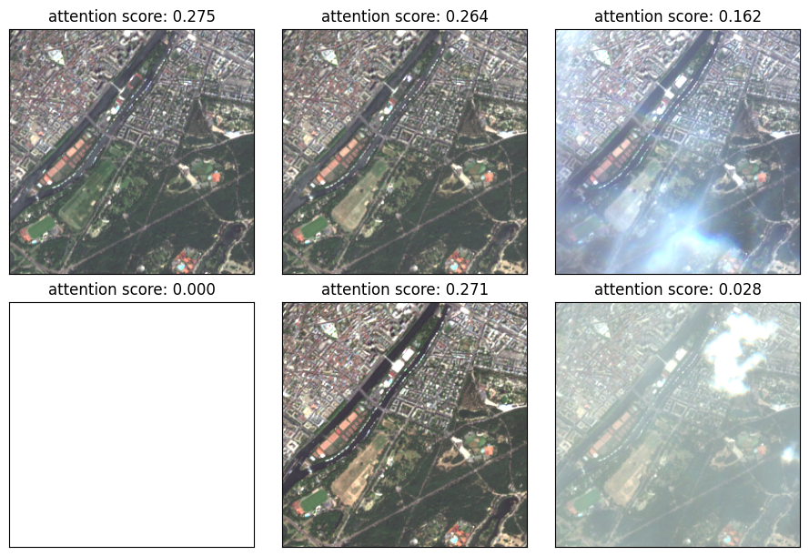
Visualize model outputs#
We can see that the model assigns lower scores to images with cloud cover, which makes intuitive sense.
For visualization, sample the same chip from the normalized RasterSource.
[20]:
x_viz = raster_source_viz.get_chip(window)
x_viz.shape
[20]:
(6, 256, 256, 3)
[92]:
T = x_viz.shape[0]
ncols = 3
nrows = int(math.ceil(T / ncols))
fig, axs = plt.subplots(
    nrows, ncols, figsize=(ncols * 3, nrows * 3), constrained_layout=True)
for ax, x_viz_t, attn_t in zip(axs.flat, x_viz, out[0]):
    ax.imshow(x_viz_t)
    ax.tick_params(top=False, bottom=False, left=False, right=False,
                labelleft=False, labelbottom=False, labeltop=False)
    ax.set_title(f'attention score: {attn_t:.3f}')
plt.show()