Quickstart#

In this Quickstart, we’ll train a semantic segmentation model on SpaceNet data. Don’t get too excited - we’ll only be training for a very short time on a very small training set! So the model that is created here will be pretty much worthless. But! These steps will show how Raster Vision pipelines are set up and run, so when you are ready to run against a lot of training data for a longer time on a GPU, you’ll know what you have to do. Also, we’ll show how to make predictions on the data using a model we’ve already trained on GPUs to show what you can expect to get out of Raster Vision.

For the Quickstart we are going to be using one of the published Docker Images as it has an environment with all necessary dependencies already installed.

The Data#

Configuring a semantic segmentation pipeline#

Create a Python file in the ${RV_QUICKSTART_CODE_DIR} named tiny_spacenet.py. Inside, you’re going to write a function called get_config that returns a SemanticSegmentationConfig object. This object’s type is a subclass of PipelineConfig, and configures a semantic segmentation pipeline which (optionally) analyzes the imagery, (optionally) creates training chips, trains a model, makes predictions on validation scenes, evaluates the predictions, and saves a model bundle.

tiny_spacenet.py#

from os.path import join
from rastervision.core.rv_pipeline import *
from rastervision.core.backend import *
from rastervision.core.data import *
from rastervision.pytorch_backend import *
from rastervision.pytorch_learner import *


def get_config(runner) -> SemanticSegmentationConfig:
    output_root_uri = '/opt/data/output/tiny_spacenet'
    class_config = ClassConfig(
        names=['building', 'background'], colors=['red', 'black'])

    base_uri = ('https://s3.amazonaws.com/azavea-research-public-data/'
                'raster-vision/examples/spacenet')
    train_image_uri = join(base_uri, 'RGB-PanSharpen_AOI_2_Vegas_img205.tif')
    train_label_uri = join(base_uri, 'buildings_AOI_2_Vegas_img205.geojson')
    val_image_uri = join(base_uri, 'RGB-PanSharpen_AOI_2_Vegas_img25.tif')
    val_label_uri = join(base_uri, 'buildings_AOI_2_Vegas_img25.geojson')

    train_scene = make_scene('scene_205', train_image_uri, train_label_uri,
                             class_config)
    val_scene = make_scene('scene_25', val_image_uri, val_label_uri,
                           class_config)
    scene_dataset = DatasetConfig(
        class_config=class_config,
        train_scenes=[train_scene],
        validation_scenes=[val_scene])

    # Use the PyTorch backend for the SemanticSegmentation pipeline.
    chip_sz = 300

    backend = PyTorchSemanticSegmentationConfig(
        data=SemanticSegmentationGeoDataConfig(
            scene_dataset=scene_dataset,
            sampling=WindowSamplingConfig(
                # randomly sample training chips from scene
                method=WindowSamplingMethod.random,
                # ... of size chip_sz x chip_sz
                size=chip_sz,
                # ... and at most 10 chips per scene
                max_windows=10)),
        model=SemanticSegmentationModelConfig(backbone=Backbone.resnet50),
        solver=SolverConfig(lr=1e-4, num_epochs=1, batch_sz=2))

    return SemanticSegmentationConfig(
        root_uri=output_root_uri,
        dataset=scene_dataset,
        backend=backend,
        predict_options=SemanticSegmentationPredictOptions(chip_sz=chip_sz))


def make_scene(scene_id: str, image_uri: str, label_uri: str,
               class_config: ClassConfig) -> SceneConfig:
    """Define a Scene with image and labels from the given URIs."""

    raster_source = RasterioSourceConfig(
        uris=image_uri,
        # use only the first 3 bands
        channel_order=[0, 1, 2],
    )

    # configure GeoJSON reading
    vector_source = GeoJSONVectorSourceConfig(
        uris=label_uri,
        # The geoms in the label GeoJSON do not have a "class_id" property, so
        # classes must be inferred. Since all geoms are for the building class,
        # this is easy to do: we just assign the building class ID to all of
        # them.
        transformers=[
            ClassInferenceTransformerConfig(
                default_class_id=class_config.get_class_id('building'))
        ])
    # configure transformation of vector data into semantic segmentation labels
    label_source = SemanticSegmentationLabelSourceConfig(
        # semantic segmentation labels must be rasters, so rasterize the geoms
        raster_source=RasterizedSourceConfig(
            vector_source=vector_source,
            rasterizer_config=RasterizerConfig(
                # What about pixels outside of any geoms? Mark them as
                # background.
                background_class_id=class_config.get_class_id('background'))))

    return SceneConfig(
        id=scene_id,
        raster_source=raster_source,
        label_source=label_source,
    )

Running the pipeline#

We can now run the pipeline by invoking the following command inside the container.

> rastervision run local code/tiny_spacenet.py

Seeing Results#

If you go to ${RV_QUICKSTART_OUT_DIR}/tiny_spacenet you should see a directory structure like this.

Note

This uses the tree command which you may need to install first.

> tree -L 3
├── Makefile
├── bundle
│   └── model-bundle.zip
├── eval
│   └── validation_scenes
│       └── eval.json
├── pipeline-config.json
├── predict
│   └── scene_25
│       └── labels.tif
└── train
    ├── dataloaders
    │   ├── train.png
    │   └── valid.png
    ├── last-model.pth
    ├── learner-config.json
    ├── log.csv
    ├── model-bundle.zip
    ├── tb-logs
    │   ├── events.out.tfevents.1670510483.c5c1c7621fb7.1830.0
    │   ├── events.out.tfevents.1670511197.c5c1c7621fb7.2706.0
    │   └── events.out.tfevents.1670595249.986730ccbe70.7507.0
    ├── valid_metrics.json
    └── valid_preds.png

Note

The numbers in your events.out.tfevents filename will not necessarily match the ones above.

The root directory contains a serialized JSON version of the configuration at pipeline-config.json, and each subdirectory with a command name contains output for that command. You can see test predictions on a batch of data in train/test_preds.png, and evaluation metrics in eval/eval.json, but don’t get too excited! We trained a model for 1 epoch on a tiny dataset, and the model is likely making random predictions at this point. We would need to train on a lot more data for a lot longer for the model to become good at this task.

Model Bundles#

To immediately use Raster Vision with a fully trained model, one can make use of the pretrained models in our Model Zoo. However, be warned that these models probably won’t work well on imagery taken in a different city, with a different ground sampling distance, or different sensor.

For example, to use a DeepLab/Resnet50 model that has been trained to do building segmentation on Las Vegas, one can type:

> rastervision predict \
    https://s3.amazonaws.com/azavea-research-public-data/raster-vision/examples/model-zoo-0.30/spacenet-vegas-buildings-ss/model-bundle.zip \
    https://s3.amazonaws.com/azavea-research-public-data/raster-vision/examples/model-zoo-0.30/spacenet-vegas-buildings-ss/sample-predictions/sample-img-spacenet-vegas-buildings-ss.tif \
    prediction

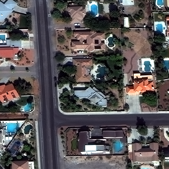
This will make predictions on the image sample-img-spacenet-vegas-buildings-ss.tif using the provided model bundle. The predictions will be stored in the prediction/ directory and will comprise a raster of predicted labels (prediction/labels.tif) and vectorized labels as GeoJSON files for each class (in prediction/vector_outputs/). These raster predictions are in the GeoTiff format, and you will need a GIS viewer such as QGIS to open them correctly on your device. Notice that the prediction package and the input raster are transparently downloaded via HTTP.

The input image (false color) and predictions are reproduced below.

Next Steps#

This is just a quick example of a Raster Vision pipeline. For several complete example of how to train models on open datasets (including SpaceNet), optionally using GPUs on AWS Batch, see the Examples.