Note

This page was generated from reading_labels.ipynb.

Note

If running outside of the Docker image, you may need to set some environment variables manually. You can do it like so:

import os
from subprocess import check_output

os.environ['GDAL_DATA'] = check_output('pip show rasterio | grep Location | awk \'{print $NF"/rasterio/gdal_data/"}\'', shell=True).decode().strip()

We will be accessing files on S3 in this notebook. Since those files are public, we set the AWS_NO_SIGN_REQUEST to tell rasterio to skip the sign-in.

%env AWS_NO_SIGN_REQUEST=YES

Reading labels

ClassConfig

Before we can work with labels, we first want to define what our target classes are – their names, their IDs, and possibly, their colors (to use for visualization).

Raster Vision makes all this simple to do using the handy ClassConfig class.

from rastervision.core.data import ClassConfig

class_config = ClassConfig(names=['background', 'foreground'])
class_config

ClassConfig(names=['background', 'foreground'], colors=[(74, 233, 235), (11, 186, 220)], null_class=None)

(Note how a unique color was generated for each class.)

The numeric ID of each class is its index in the names list.

We can query the ID of a class like so:

print('background', class_config.get_class_id('background'))
print('foreground', class_config.get_class_id('foreground'))

background 0
foreground 1

In the example above, ClassConfig automatically generated a color for each class. We could have instead manually specified them. The colors can be any color-string recognized by PIL.

class_config = ClassConfig(
    names=['background', 'foreground'],
    colors=['lightgray', 'darkred'])
class_config

ClassConfig(names=['background', 'foreground'], colors=['lightgray', 'darkred'], null_class=None)

---

The “null” class

Geospatial rasters can have NODATA pixels. This is relevant for semantic segmentation where you need to assign a label to every pixel.

You may either want to assign them a class of their own or consider them a part of a catch-all “background” class.

ClassConfig’s name for this class is the “null class”. Below are some ways that you can define it.

1. Designate one class as the “null” class.

class_config = ClassConfig(names=['background', 'foreground'], null_class='background')
class_config

ClassConfig(names=['background', 'foreground'], colors=[(20, 52, 212), (160, 39, 55)], null_class='background')

2. Specify a class called “null”.

class_config = ClassConfig(names=['null', 'foreground'])
class_config

ClassConfig(names=['null', 'foreground'], colors=[(174, 196, 28), (152, 158, 202)], null_class='null')

3. Call .ensure_null_class() to automatically add an additional “null” class.

class_config = ClassConfig(names=['background', 'foreground'])
class_config.ensure_null_class()
class_config

ClassConfig(names=['background', 'foreground', 'null'], colors=[(135, 60, 187), (31, 100, 192), 'black'], null_class='null')

---

Normalized colors

Another nifty functionality is the color_triples property that returns the colors in a normalized form that can be directly used with matplotlib.

The example below shows how we can easily create a color-map from our class colors.

from matplotlib.colors import ListedColormap

class_config = ClassConfig(names=['a', 'b', 'c', 'd', 'e', 'f'])
cmap = ListedColormap(class_config.color_triples)
cmap

from_list

under

bad

over

---

LabelSource

While RasterSources and VectorSources allow us to read raw data, the LabelSources take this data and convert them into a form suitable for machine learning.

We have 3 kinds of pre-defined LabelSources – one for each of the 3 main computer vision tasks: semantic segmentation, object detection, and chip classification.

---

Semantic Segmentation - SemanticSegmentationLabelSource

SemanticSegmentationLabelSource is perhaps the simplest of LabelSources. Since semantic segmentation labels are rasters themselves, SemanticSegmentationLabelSource takes in a RasterSource and allows querying chips from it using array-indexing or Box's.

The main added service it provides is ensuring that if a chip overflows the extent, the overflowing pixels are assigned the ID of the “null class”.

---

The example below shows how to create a SemanticSegmentationLabelSource from rasterized vector labels.

img_uri = 's3://azavea-research-public-data/raster-vision/examples/spacenet/RGB-PanSharpen_AOI_2_Vegas_img205.tif'
label_uri = 's3://azavea-research-public-data/raster-vision/examples/spacenet/buildings_AOI_2_Vegas_img205.geojson'

Define ClassConfig:

from rastervision.core.data import ClassConfig

class_config = ClassConfig(
    names=['background', 'building'],
    colors=['lightgray', 'darkred'],
    null_class='background')

Create

• a RasterSource to get the image extent and a CRSTransformer

• a VectorSource to read the vector labels

• a RasterizedSource to rasterize the VectorSource

from rastervision.core.data import (
    ClassInferenceTransformer, GeoJSONVectorSource,
    RasterioSource, RasterizedSource)

img_raster_source = RasterioSource(img_uri, allow_streaming=True)

vector_source = GeoJSONVectorSource(
    label_uri,
    img_raster_source.crs_transformer,
    vector_transformers=[
        ClassInferenceTransformer(
            default_class_id=class_config.get_class_id('building'))])

label_raster_source = RasterizedSource(
    vector_source,
    background_class_id=class_config.null_class_id,
    bbox=img_raster_source.bbox)

2024-04-09 19:56:03:rastervision.pipeline.file_system.utils: INFO - Using cached file /opt/data/tmp/cache/s3/azavea-research-public-data/raster-vision/examples/spacenet/buildings_AOI_2_Vegas_img205.geojson.

Create a SemanticSegmentationLabelSource from the RasterizedSource.

from rastervision.core.data import SemanticSegmentationLabelSource

label_source = SemanticSegmentationLabelSource(
    label_raster_source, class_config=class_config)

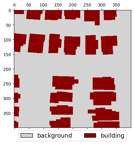
We can sample label-chips like so:

label_chip = label_source[:400, :400]

## equivalent to:
#
# from rastervision.core.box import Box
# label_chip = label_source.get_label_arr(Box(0, 0, 400, 400))

from matplotlib import pyplot as plt
from matplotlib.colors import ListedColormap
from matplotlib import patches

fig, ax = plt.subplots(figsize=(5, 5))
cmap = ListedColormap(class_config.color_triples)
ax.matshow(label_chip, cmap=cmap)

legend_items = [
    patches.Patch(facecolor=cmap(i), edgecolor='black', label=cname)
    for i, cname in enumerate(class_config.names)]
ax.legend(
    handles=legend_items,
    ncol=len(class_config),
    loc='upper center',
    fontsize=14,
    bbox_to_anchor=(0.5, 0))
plt.show()

---

Object Detection - ObjectDetectionLabelSource

The ObjectDetectionLabelSource allows querying all the label bounding boxes and their corresponding class IDs that fall inside a window. It also transforms the coordinates of the returned bounding boxes so that they represent points inside the window rather than the global extent.

The bounding-box-to-window matching behavior can be further controlled by specifying an ioa_thresh (intersection-over-area threshold for considering a bounding box a part of a window) and a clip flag which ensures that bounding boxes do not overflow the window.

---

Download (~500 KB) and unzip data:

!wget "https://github.com/azavea/raster-vision-data/releases/download/v0.0.1/cowc-potsdam-labels.zip" -P "data"
!apt install unzip
!unzip "data/cowc-potsdam-labels.zip" -d "data/cowc-potsdam-labels/"

img_uri = 's3://azavea-research-public-data/raster-vision/examples/tutorials-data/top_potsdam_2_10_RGBIR.tif'
label_uri = 'data/cowc-potsdam-labels/labels/train/top_potsdam_2_10_RGBIR.json'

Create - a RasterSource to get the image extent and a CRSTRansformer - a VectorSource to read the vector labels - an ObjectDetectionLabelSource to convert data from VectorSource into object detection labels

from rastervision.core.data import (
    ClassConfig, ClassInferenceTransformer, GeoJSONVectorSource,
    ObjectDetectionLabelSource, RasterioSource)

class_config = ClassConfig(names=['car'], colors=['red'])

raster_source = RasterioSource(img_uri, allow_streaming=True)

vector_source = GeoJSONVectorSource(
    label_uri,
    crs_transformer=raster_source.crs_transformer,
    vector_transformers=[
        ClassInferenceTransformer(
            default_class_id=class_config.get_class_id('car'))])

label_source = ObjectDetectionLabelSource(
    vector_source, bbox=raster_source.bbox, ioa_thresh=0.2, clip=False)

Warning 1: TIFFReadDirectory:Sum of Photometric type-related color channels and ExtraSamples doesn't match SamplesPerPixel. Defining non-color channels as ExtraSamples.

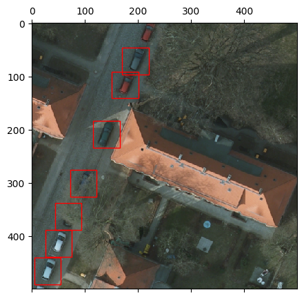
We can sample label data like shown below. Here, we are querying a 1000x1000 chip downscaled by a factor of 2 from the raster source. Using the same index for the ObjectDetectionLabelSource gets us all the bounding boxes that fall within the 1000x1000 window and are automatically downscaled by a factor of 2 so that they still align correctly with the image chip.

chip = raster_source[:1000:2, :1000:2]
bboxes, _, _ = label_source[:1000:2, :1000:2]

from matplotlib import pyplot as plt
from matplotlib import patches as patches
import numpy as np
from shapely.geometry import Polygon

fig, ax = plt.subplots(figsize=(5, 5))

ax.matshow(chip[..., :3])

bbox_color = class_config.color_triples[class_config.get_class_id('car')]
bbox_polygons = [Polygon.from_bounds(*bounds) for bounds in bboxes[:, [1, 0, 3, 2]]]
for p in bbox_polygons:
    xy = np.array(p.exterior.coords)
    patch = patches.Polygon(xy, fill=None, color=bbox_color)
    ax.add_patch(patch)
ax.autoscale()

plt.show()

---

Chip Classification - ChipClassificationLabelSource

The ChipClassificationLabelSource can do the following:

1. The trivial case: given a rectangular polygons (representing chips) with associated class IDs, allow querying the class ID for those chips.

2. The more interesting case: given polygons representing the members of the target class(es), infer the class ID for a window based on how much it overlaps with any label-polygon.

The example below showcases the latter.

---

Data source: SpaceNet 1

Warning

This example will download a 150 MB file.

img_uri = 's3://spacenet-dataset/AOIs/AOI_1_Rio/srcData/mosaic_3band/013022232020.tif'
label_uri = 's3://spacenet-dataset/AOIs/AOI_1_Rio/srcData/buildingLabels/Rio_Buildings_Public_AOI_v2.geojson'

Create - a RasterSource to get the image extent and a CRSTRansformer - a VectorSource to read the vector labels

from rastervision.core.data import (
    ClassConfig, ClassInferenceTransformer,
    GeoJSONVectorSource, RasterioSource)

class_config = ClassConfig(
    names=['background', 'building'], null_class='background')

raster_source = RasterioSource(img_uri, allow_streaming=True)

vector_source = GeoJSONVectorSource(
    label_uri,
    crs_transformer=raster_source.crs_transformer,
    vector_transformers=[
        ClassInferenceTransformer(
            default_class_id=class_config.get_class_id('building'))])

ChipClassificationLabelSource accepts a number of options for configuring the class ID inference behavior. These must be specified through the ChipClassificationLabelSourceConfig.

from rastervision.core.data import (
    ChipClassificationLabelSource, ChipClassificationLabelSourceConfig)

cfg = ChipClassificationLabelSourceConfig(
    ioa_thresh=0.5,
    use_intersection_over_cell=False,
    pick_min_class_id=False,
    background_class_id=class_config.null_class_id,
    infer_cells=True)

label_source = ChipClassificationLabelSource(
    cfg, vector_source, bbox=raster_source.bbox, lazy=True)

2024-04-09 19:58:55:rastervision.pipeline.file_system.utils: INFO - Downloading s3://spacenet-dataset/AOIs/AOI_1_Rio/srcData/buildingLabels/Rio_Buildings_Public_AOI_v2.geojson to /opt/data/tmp/cache/s3/spacenet-dataset/AOIs/AOI_1_Rio/srcData/buildingLabels/Rio_Buildings_Public_AOI_v2.geojson...

---

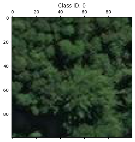
We can query ChipClassificationLabelSourceConfig in the usual way. For a given index/window, ChipClassificationLabelSourceConfig retuns a single int representing the class ID of the inferred class of that chip.

Querying a 100x100 chip from the corner of the raster, we see that there are no buildings, and indeed the label returned corresponds to the "background" class.

from matplotlib import pyplot as plt

chip = raster_source[:100, :100]
label = label_source[:100, :100]

fig, ax = plt.subplots(figsize=(5, 5))
ax.matshow(chip)
ax.set_title(f'Class ID: {label}')
plt.show()

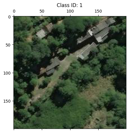
Querying a different chip, we see that it does in fact contain buildings, and the label source agrees – returning the label corresponding to the "building" class.

from matplotlib import pyplot as plt

chip = raster_source[:200, 200:400]
label = label_source[:200, 200:400]

fig, ax = plt.subplots(figsize=(5, 5))
ax.matshow(chip)
ax.set_title(f'Class ID: {label}')
plt.show()

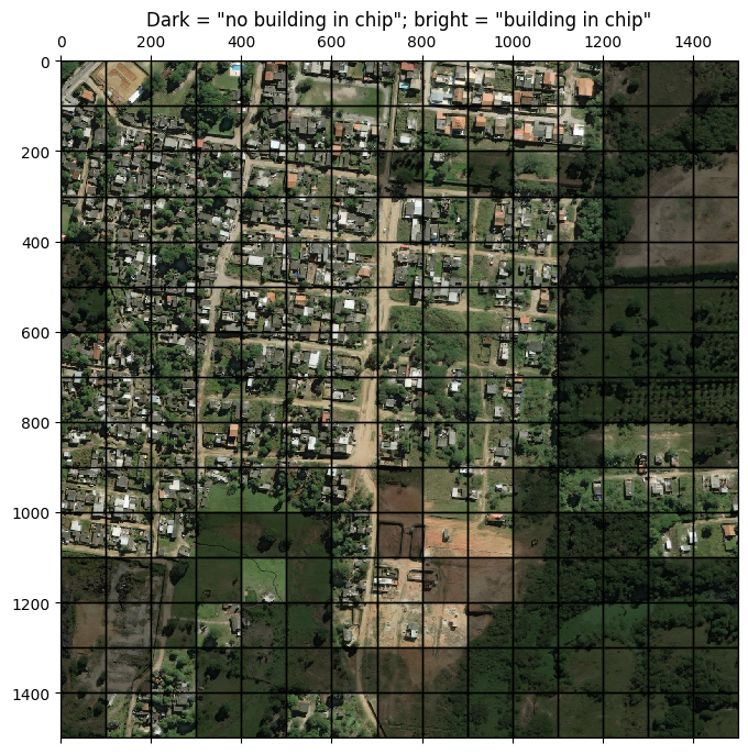
To get a better sense of ChipClassificationLabelSource’s working we will now query the class for many 100x100 chips within a 1500x1500 chunk of the full raster.

from matplotlib import pyplot as plt
from matplotlib import patches as patches
import numpy as np
from shapely.geometry import Polygon
from rastervision.core.box import Box

chip = raster_source[500:2000, 500:2000]

extent = Box(500, 500, 2000, 2000)
windows = extent.get_windows(100, stride=100)
label_source.populate_labels(cells=windows)

fig, ax = plt.subplots(figsize=(8, 8))
ax.matshow(chip[..., :3])

for w in windows:
    p = w.translate(-500, -500).to_shapely()
    xy = np.array(p.exterior.coords)
    label = label_source[w] # equivalent to label_source[w.ymin:w.ymax, w.xmin:w.xmax]
    if label == 0:
        patch = patches.Polygon(xy, fc='k', alpha=0.45)
        ax.add_patch(patch)
        patch = patches.Polygon(xy, fill=None, ec='k', alpha=1, lw=1)
    else:
        patch = patches.Polygon(xy, fill=None, ec='k', alpha=1, lw=1)
    ax.add_patch(patch)
ax.set_title('Dark = "no building in chip"; bright = "building in chip"')
plt.show()

---

Labels

The Labels class is a source-agnostic, in-memory representation of the labels in a scene.

We can get all or a subset of a LabelSource as a Labels instance, by calling LabelSource.get_labels(). E.g.

labels = label_source.get_labels(window)

Crucially, the predictions produced by a model can also be converted to Labels instance, allowing them to be compared agains the Labels from the LabelSource (i.e, the ground truth) to get performance metrics. This is essentially what Evaluator does.

There is one for each of the three tasks:

• ChipClassificationLabels

• SemanticSegmentationLabels

• ObjectDetectionLabels