Note
This page was generated from lightning_workflow.ipynb.
Note
If running outside of the Docker image, you may need to set some environment variables manually. You can do it like so:
import os
from subprocess import check_output

os.environ['GDAL_DATA'] = check_output('pip show rasterio | grep Location | awk \'{print $NF"/rasterio/gdal_data/"}\'', shell=True).decode().strip()
We will be accessing files on S3 in this notebook. Since those files are public, we set the AWS_NO_SIGN_REQUEST to tell rasterio to skip the sign-in.
[1]:
%env AWS_NO_SIGN_REQUEST=YES
env: AWS_NO_SIGN_REQUEST=YES
Using Raster Vision with Lightning#
![]()
Lightning (formerly known as PyTorch Lightning) is a high-level library for training PyTorch models. In this tutorial, we demonstrate a complete workflow for doing semantic segmentation on SpaceNet Vegas using a combination of Raster Vision and Lightning. We use Raster Vision for reading data, Lightning for training a model, and then Raster Vision again for making predictions and evaluations on whole scenes.
Raster Vision has easy-to-use, built-in model training functionality implemented by the Learner class which is shown in the “Training a model” tutorial. However, some users may prefer to use Lightning for training models, either because they already know how to use it, and like it, or because they desire more flexibility than the Learner class offers. This notebook shows how these libraries can be used together, but does not attempt to use either library in a
particularly sophisticated manner.
First, we need to install pytorch-lightning since it is not a dependency of Raster Vision.
[ ]:
%pip install -q pytorch-lightning==2.*
Define training and validation datasets#
We use Raster Vision to create training and validation Dataset objects. To keep things simple, we use a single scene for training and the same for validation. In a real workflow we would use many more scenes.
[3]:
import albumentations as A

from rastervision.pytorch_learner import (
    SemanticSegmentationRandomWindowGeoDataset,
    SemanticSegmentationSlidingWindowGeoDataset,
    SemanticSegmentationVisualizer)
from rastervision.core.data import ClassConfig, StatsTransformer
[4]:
scene_id = 5631
train_image_uri = f's3://spacenet-dataset/spacenet/SN2_buildings/train/AOI_2_Vegas/PS-RGB/SN2_buildings_train_AOI_2_Vegas_PS-RGB_img{scene_id}.tif'
train_label_uri = f's3://spacenet-dataset/spacenet/SN2_buildings/train/AOI_2_Vegas/geojson_buildings/SN2_buildings_train_AOI_2_Vegas_geojson_buildings_img{scene_id}.geojson'

class_config = ClassConfig(
    names=['building', 'background'],
    colors=['orange', 'black'],
    null_class='background')

data_augmentation_transform = A.Compose([
    A.Flip(),
    A.ShiftScaleRotate(),
    A.RGBShift()
])

train_ds = SemanticSegmentationRandomWindowGeoDataset.from_uris(
    class_config=class_config,
    image_uri=train_image_uri,
    label_vector_uri=train_label_uri,
    label_vector_default_class_id=class_config.get_class_id('building'),
    size_lims=(200, 250),
    out_size=325,
    max_windows=10,
    transform=data_augmentation_transform,
    padding=50,
    image_raster_source_kw=dict(raster_transformers=[
        StatsTransformer(means=[562.7, 716.6, 517.1], stds=[341.1, 341.5, 197.5])
    ])
)
2024-08-07 14:05:36:rastervision.pipeline.file_system.utils: INFO - Using cached file /opt/data/tmp/cache/s3/spacenet-dataset/spacenet/SN2_buildings/train/AOI_2_Vegas/PS-RGB/SN2_buildings_train_AOI_2_Vegas_PS-RGB_img5631.tif.
INFO:rastervision.pipeline.file_system.utils:Using cached file /opt/data/tmp/cache/s3/spacenet-dataset/spacenet/SN2_buildings/train/AOI_2_Vegas/PS-RGB/SN2_buildings_train_AOI_2_Vegas_PS-RGB_img5631.tif.
2024-08-07 14:05:36:rastervision.pipeline.file_system.utils: INFO - Using cached file /opt/data/tmp/cache/s3/spacenet-dataset/spacenet/SN2_buildings/train/AOI_2_Vegas/geojson_buildings/SN2_buildings_train_AOI_2_Vegas_geojson_buildings_img5631.geojson.
INFO:rastervision.pipeline.file_system.utils:Using cached file /opt/data/tmp/cache/s3/spacenet-dataset/spacenet/SN2_buildings/train/AOI_2_Vegas/geojson_buildings/SN2_buildings_train_AOI_2_Vegas_geojson_buildings_img5631.geojson.
To check that data is being read correctly, we use the Visualizer to plot a batch.
[5]:
viz = SemanticSegmentationVisualizer(
    class_names=class_config.names, class_colors=class_config.colors)
x, y = viz.get_batch(train_ds, 4)
viz.plot_batch(x, y, show=True)

[5]:
scene_id = 5632
val_image_uri = f's3://spacenet-dataset/spacenet/SN2_buildings/train/AOI_2_Vegas/PS-RGB/SN2_buildings_train_AOI_2_Vegas_PS-RGB_img{scene_id}.tif'
val_label_uri = f's3://spacenet-dataset/spacenet/SN2_buildings/train/AOI_2_Vegas/geojson_buildings/SN2_buildings_train_AOI_2_Vegas_geojson_buildings_img{scene_id}.geojson'

val_ds = SemanticSegmentationSlidingWindowGeoDataset.from_uris(
    class_config=class_config,
    image_uri=val_image_uri,
    label_vector_uri=val_label_uri,
    label_vector_default_class_id=class_config.get_class_id('building'),
    size=325,
    stride=100,
    out_size=325,
)
2024-08-07 14:05:41:rastervision.pipeline.file_system.utils: INFO - Using cached file /opt/data/tmp/cache/s3/spacenet-dataset/spacenet/SN2_buildings/train/AOI_2_Vegas/PS-RGB/SN2_buildings_train_AOI_2_Vegas_PS-RGB_img5632.tif.
INFO:rastervision.pipeline.file_system.utils:Using cached file /opt/data/tmp/cache/s3/spacenet-dataset/spacenet/SN2_buildings/train/AOI_2_Vegas/PS-RGB/SN2_buildings_train_AOI_2_Vegas_PS-RGB_img5632.tif.
2024-08-07 14:05:41:rastervision.pipeline.file_system.utils: INFO - Using cached file /opt/data/tmp/cache/s3/spacenet-dataset/spacenet/SN2_buildings/train/AOI_2_Vegas/geojson_buildings/SN2_buildings_train_AOI_2_Vegas_geojson_buildings_img5632.geojson.
INFO:rastervision.pipeline.file_system.utils:Using cached file /opt/data/tmp/cache/s3/spacenet-dataset/spacenet/SN2_buildings/train/AOI_2_Vegas/geojson_buildings/SN2_buildings_train_AOI_2_Vegas_geojson_buildings_img5632.geojson.
Train Model using Lightning#
Here we build a DeepLab-ResNet50 model, and then train it using Lightning. We only train for 3 epochs so this can run in a minute or so on a CPU. In a real workflow we would train for 10-100 epochs on GPU. Because of this, the model will not be accurate at all.
[6]:
from tqdm.autonotebook import tqdm
import torch
from torch.utils.data import DataLoader
from torch.nn import functional as F
from torchvision.models.segmentation import deeplabv3_resnet50
import pytorch_lightning as pl

from rastervision.pipeline.file_system import make_dir
[23]:
batch_size = 8
lr = 1e-4
epochs = 3
output_dir = 'data/lightning-demo/'
make_dir(output_dir)
fast_dev_run = False
[8]:
train_dl = DataLoader(train_ds, batch_size=batch_size, shuffle=True, num_workers=4)
val_dl = DataLoader(val_ds, batch_size=batch_size, num_workers=4)
One of the main abstractions in Lightning is the LightningModule which extends a PyTorch nn.Module with extra methods that define how to train and validate the model. Here we define a LightningModule that does the bare minimum to train a DeepLab semantic segmentation model.
[9]:
class SemanticSegmentation(pl.LightningModule):
    def __init__(self, deeplab, lr=1e-4):
        super().__init__()
        self.deeplab = deeplab
        self.lr = lr

    def forward(self, img):
        return self.deeplab(img)['out']

    def training_step(self, batch, batch_idx):
        img, mask = batch
        img = img.float()
        mask = mask.long()
        out = self.forward(img)
        loss = F.cross_entropy(out, mask)
        log_dict = {'train_loss': loss}
        self.log_dict(log_dict, on_step=True, on_epoch=True, prog_bar=True, logger=True)
        return loss

    def validation_step(self, batch, batch_idx):
        img, mask = batch
        img = img.float()
        mask = mask.long()
        out = self.forward(img)
        loss = F.cross_entropy(out, mask)
        log_dict = {'validation_loss': loss}
        self.log_dict(log_dict, on_step=True, on_epoch=True, prog_bar=True, logger=True)
        return loss

    def configure_optimizers(self):
        optimizer = torch.optim.Adam(
            self.parameters(), lr=self.lr)
        return optimizer
The other main abstraction in Lighting is the Trainer which is responsible for actually training a LightningModule. This is configured to log metrics to Tensorboard.
[15]:
from pytorch_lightning.loggers import CSVLogger, TensorBoardLogger

deeplab = deeplabv3_resnet50(num_classes=len(class_config))
model = SemanticSegmentation(deeplab, lr=lr)
tb_logger = TensorBoardLogger(save_dir=output_dir, flush_secs=10)
trainer = pl.Trainer(
    accelerator='auto',
    min_epochs=1,
    max_epochs=epochs+1,
    default_root_dir=output_dir,
    logger=[tb_logger],
    fast_dev_run=fast_dev_run,
    log_every_n_steps=1,
)
INFO:pytorch_lightning.utilities.rank_zero:GPU available: True (cuda), used: True
INFO:pytorch_lightning.utilities.rank_zero:TPU available: False, using: 0 TPU cores
INFO:pytorch_lightning.utilities.rank_zero:HPU available: False, using: 0 HPUs
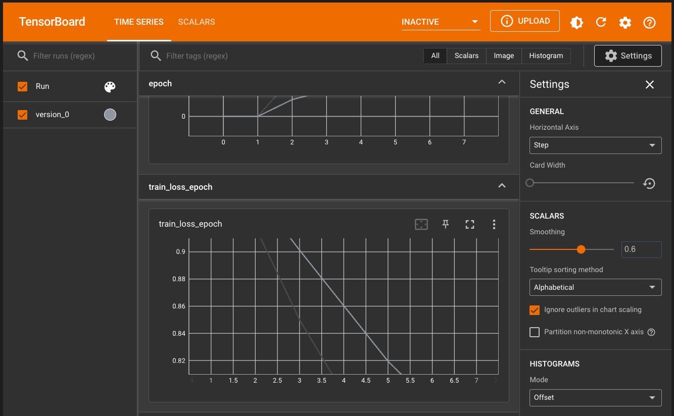
Monitor training using Tensorboard#
This runs an instance of Tensorboard inside this notebook.
Note
If running inside the Raster Vision docker image, you will need to pass –tensorboard to docker/run for this to work.
If the dashboard doen’t auto-reload, you can click the reload button on the top-right.
[ ]:
%reload_ext tensorboard
%tensorboard --bind_all --logdir "./lightning-demo/lightning_logs" --reload_interval 10
[12]:
trainer.fit(model, train_dl, val_dl)
You are using a CUDA device ('NVIDIA GeForce RTX 4080 Laptop GPU') that has Tensor Cores. To properly utilize them, you should set `torch.set_float32_matmul_precision('medium' | 'high')` which will trade-off precision for performance. For more details, read https://pytorch.org/docs/stable/generated/torch.set_float32_matmul_precision.html#torch.set_float32_matmul_precision
Missing logger folder: ./lightning-demo/lightning_logs
LOCAL_RANK: 0 - CUDA_VISIBLE_DEVICES: [0]

  | Name    | Type      | Params
--------------------------------------
0 | deeplab | DeepLabV3 | 39.6 M
--------------------------------------
39.6 M    Trainable params
0         Non-trainable params
39.6 M    Total params
158.537   Total estimated model params size (MB)
`Trainer.fit` stopped: `max_epochs=4` reached.
Load saved model#
After training the model for only 3 epochs, it will not make good predictions. In order to have some sensible looking output, we will loads weights from a model that was fully trained on SpaceNet Vegas.
[16]:
weights_uri = 'https://s3.amazonaws.com/azavea-research-public-data/raster-vision/examples/model-zoo-0.31/spacenet-vegas-buildings-ss/train/last-model.pth'
state_dict = torch.hub.load_state_dict_from_url(weights_uri, map_location='cpu')
model.deeplab.load_state_dict(state_dict)
[16]:
<All keys matched successfully>
Load normalization stats#
The model expects images to be normalized, so we load the stats needed to do that:
[17]:
from rastervision.core.data import StatsTransformer

stats_uri = 's3://azavea-research-public-data/raster-vision/examples/model-zoo-0.31/spacenet-vegas-buildings-ss/analyze/stats/train_scenes/stats.json'
stats_tf = StatsTransformer.from_stats_json(stats_uri)
stats_tf
[17]:
StatsTransformer(means=array([424.87790094, 592.92457995, 447.27932498]), stds=array([220.60852518, 242.79340345, 148.50591309]), max_stds=3.0)
Next, we re-initialize val_ds and val_dl to make use of the stats. Note that we skip passing the class_config and label URI, since we will not be using this for training.
[18]:
val_ds = SemanticSegmentationSlidingWindowGeoDataset.from_uris(
    image_uri=val_image_uri,
    image_raster_source_kw=dict(raster_transformers=[stats_tf]),
    size=325,
    stride=325,
    out_size=325,
)
val_dl = DataLoader(val_ds, batch_size=batch_size, num_workers=4)
2024-08-07 14:11:08:rastervision.pipeline.file_system.utils: INFO - Using cached file /opt/data/tmp/cache/s3/spacenet-dataset/spacenet/SN2_buildings/train/AOI_2_Vegas/PS-RGB/SN2_buildings_train_AOI_2_Vegas_PS-RGB_img5632.tif.
INFO:rastervision.pipeline.file_system.utils:Using cached file /opt/data/tmp/cache/s3/spacenet-dataset/spacenet/SN2_buildings/train/AOI_2_Vegas/PS-RGB/SN2_buildings_train_AOI_2_Vegas_PS-RGB_img5632.tif.
Make predictions for scene#
We can now use Raster Vision’s SemanticSegmentationLabels class to make predictions over a whole scene. The SemanticSegmentationLabels.from_predictions() method takes an iterator over predictions. We create this using a get_predictions() helper function defined below.
[19]:
def get_predictions(dataloader):
    for x, _ in tqdm(dataloader):
        with torch.inference_mode():
            out_batch = model(x)
            out_batch = out_batch.softmax(dim=1)
        # This needs to yield a single prediction, not a whole batch of them.
        for out in out_batch:
            yield out.numpy()
[20]:
from rastervision.core.data import SemanticSegmentationLabels

model.eval()
predictions = get_predictions(val_dl)
pred_labels = SemanticSegmentationLabels.from_predictions(
    val_ds.windows,
    predictions,
    smooth=True,
    extent=val_ds.scene.extent,
    num_classes=len(class_config),
)
scores = pred_labels.get_score_arr(pred_labels.extent)
Visualize and then save predictions#
[21]:
from matplotlib import pyplot as plt

scores_building = scores[0]
scores_background = scores[1]

fig, (ax1, ax2) = plt.subplots(1, 2, figsize=(10, 5))
fig.tight_layout(w_pad=-2)
ax1.imshow(scores_building, cmap='plasma')
ax1.axis('off')
ax1.set_title('building')
ax2.imshow(scores_background, cmap='plasma')
ax2.axis('off')
ax2.set_title('background')
plt.show()

[24]:
from os.path import join

pred_labels.save(
    uri=join(output_dir, 'predictions'),
    crs_transformer=val_ds.scene.raster_source.crs_transformer,
    class_config=class_config)
What next?#
See the Evaluate predictions tutorial to see how to compute performance metrics for these predictions.