Pipelines and Commands#
In addition to providing abstract pipeline functionality, Raster Vision provides a set of concrete pipelines for deep learning on remote sensing imagery including ChipClassification, SemanticSegmentation, and ObjectDetection. These pipelines all derive from RVPipeline, and are provided by the rastervision.core package. It’s possible to customize these pipelines as well as create new ones from scratch, which is discussed in Customizing Raster Vision.
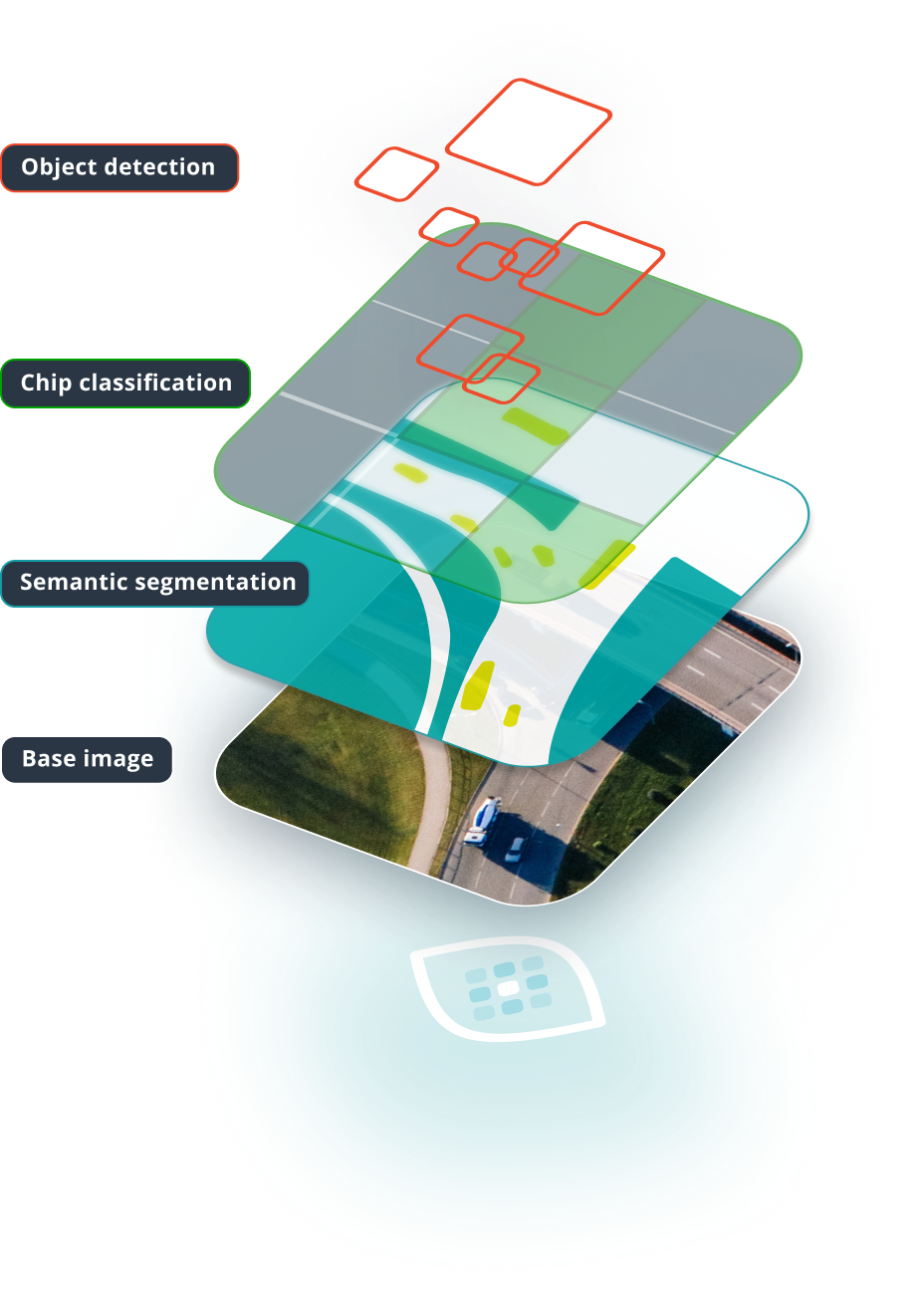
Chip Classification#
In chip classification, the goal is to divide the scene up into a grid of cells and classify each cell. This task is good for getting a rough idea of where certain objects are located, or where indiscrete “stuff” (such as grass) is located. It requires relatively low labeling effort, but also produces spatially coarse predictions. In our experience, this task trains the fastest, and is easiest to configure to get “decent” results.
Object Detection#
In object detection, the goal is to predict a bounding box and a class around each object of interest. This task requires higher labeling effort than chip classification, but has the ability to localize and individuate objects. Object detection models require more time to train and also struggle with objects that are very close together. In theory, it is straightforward to use object detection for counting objects.
Semantic Segmentation#
In semantic segmentation, the goal is to predict the class of each pixel in a scene. This task requires the highest labeling effort, but also provides the most spatially precise predictions. Like object detection, these models take longer to train than chip classification models.
Configuring RVPipelines#
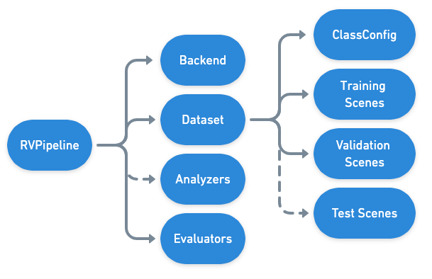
Each (subclass of) RVPipeline is configured by returning an instance of (a subclass of) RVPipelineConfigs from a get_config() function in a Python module. It’s also possible to return a list of RVPipelineConfigs from get_configs(), which will be executed in parallel.
Each RVPipelineConfig object specifies the details about how the commands within the pipeline will execute (ie. which files, what methods, what hyperparameters, etc.). In contrast, the pipeline runner, which actually executes the commands in the pipeline, is specified as an argument to the Command Line Interface. The following diagram shows the hierarchy of the high level components comprising an RVPipeline:
In the tiny_spacenet.py example, the SemanticSegmentationConfig is the last thing constructed and returned from the get_config function.
return SemanticSegmentationConfig(
    root_uri=output_root_uri,
    dataset=scene_dataset,
    backend=backend,
    predict_options=SemanticSegmentationPredictOptions(chip_sz=chip_sz))
See also
The ChipClassificationConfig, SemanticSegmentationConfig, and ObjectDetectionConfig API docs have more information on configuring pipelines.
Commands#
The RVPipelines provide a sequence of commands, which are described below.
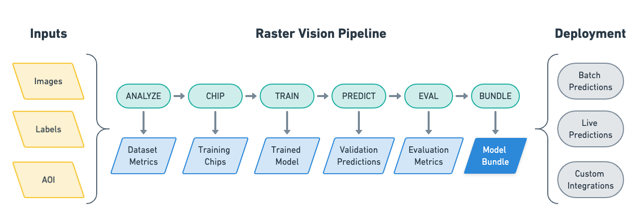
ANALYZE#
The ANALYZE command is used to analyze scenes that are part of an experiment and produce some output that can be consumed by later commands. Geospatial raster sources such as GeoTIFFs often contain 16- and 32-bit pixel color values, but many deep learning libraries expect 8-bit values. In order to perform this transformation, we need to know the distribution of pixel values. So one usage of the ANALYZE command is to compute statistics of the raster sources and save them to a JSON file which is later used by the StatsTransformer (one of the available RasterTransformers) to do the conversion.
CHIP#
Scenes comprise large geospatial raster sources (e.g. GeoTIFFs) and geospatial label sources (e.g. GeoJSONs), but models can only consume small images (i.e. chips) and labels in pixel based-coordinates. In addition, each Backend has its own dataset format. The CHIP command solves this problem by converting scenes into training chips and into a format the backend can use for training.
TRAIN#
The TRAIN command is used to train a model using the dataset generated by the CHIP command. The command uses the Backend to run a training loop that saves the model and other artifacts each epoch. If the training command is interrupted, it will resume at the last epoch when restarted.
PREDICT#
The PREDICT command makes predictions for a set of scenes using a model produced by the TRAIN command. To do this, a sliding window is used to feed small images into the model, and the predictions are transformed from image-centric, pixel-based coordinates into scene-centric, map-based coordinates.
EVAL#
The EVAL command evaluates the quality of models by comparing the predictions generated by the PREDICT command to ground truth labels. A variety of metrics including F1, precision, and recall are computed for each class (as well as overall) and are written to a JSON file.
Pipeline components#
Below we describe some components of the pipeline that you might directly or indirectly configure.
A lot of these will be familiar from Basic Concepts, but note that when configuring a pipeline, instead of dealing with the classes directly, you will instead be configuring their Config counterparts.
Configs#
A Config is a Raster Vision class based on the pydantic BaseModel class that allows various kinds of configurations to be stored in a systematic, typed, validatable, and serializable way. Most of these also implement a build() method that allows the corresponding object to be created based on the configuration. For example, RasterioSourceConfig.build() builds a RasterioSource object.
Note
Configs and backward compatibility
Another crucial role that Configs play is enabling backward compatibility. Suppose you trained a model and stored it in a model-bundle using an older version of Raster Vision, and now want to use that bundle with a newer version of Raster Vision installed. This can be a problem if the specification of any Configs has changed between the two versions (e.g. if a field was removed or renamed), which means the newer version will not be able to deserialize the older pipeline config stored in the bundle.
Raster Vision solves this issue by associating each Raster Vision plugin with a version number (this is distinct from the Python package version) and providing a config-upgrader mechanism. You can define an upgrader function that takes as input the serialized config dict and a version number and modifies the dict in such a way that makes it compatible with the current version. This function is called multiple times for each config–once for each version number, from zero to the current version. An example upgrader function is shown below.
def rs_config_upgrader(cfg_dict: dict, version: int) -> dict:
   if version == 6:
      # removed in version 7
      if cfg_dict.get('extent_crop') is not None:
            raise ConfigError('RasterSourceConfig.extent_crop is deprecated.')
      try:
            del cfg_dict['extent_crop']
      except KeyError:
            pass
   elif version == 9:
      # renamed in version 10
      cfg_dict['bbox'] = cfg_dict.get('extent')
      try:
            del cfg_dict['extent']
      except KeyError:
            pass
   return cfg_dict
This upgrader function can then be registered against the corresponding Config by passing it to the upgrader= keyword argument in register_config() as shown below.
@register_config('raster_source', upgrader=rs_config_upgrader)
class RasterSourceConfig(Config):
   ...
The following table shows the corresponding Config counterparts for various commonly used classes.
Class |
Config |
Notes |
|---|---|---|
Backend#
RVPipelines use a “backend” abstraction inspired by Keras, which makes it easier to customize the code for building and training models (including using Raster Vision with arbitrary deep learning libraries).
Each backend is a subclass of Backend and has methods for saving training chips, training models, and making predictions, and is configured with a ~Backend.
The rastervision.pytorch_backend plugin provides backends that are thin wrappers around the rastervision.pytorch_learner package, which does most of the heavy lifting of building and training models using torch and torchvision. (Note that rastervision.pytorch_learner is decoupled from rastervision.pytorch_backend so that it can be used in conjunction with rastervision.pipeline to write arbitrary computer vision pipelines that have nothing to do with remote sensing.)
Here are the PyTorch backends:
The
PyTorchChipClassificationbackend trains classification models from torchvision.The
PyTorchObjectDetectionbackend trains the Faster-RCNN model in torchvision.The
PyTorchSemanticSegmentationbackend trains the DeepLabV3 model in torchvision.
In our tiny_spacenet.py example, we configured the PyTorch semantic segmentation backend using:
# Use the PyTorch backend for the SemanticSegmentation pipeline.
chip_sz = 300

backend = PyTorchSemanticSegmentationConfig(
    data=SemanticSegmentationGeoDataConfig(
        scene_dataset=scene_dataset,
        sampling=WindowSamplingConfig(
            # randomly sample training chips from scene
            method=WindowSamplingMethod.random,
            # ... of size chip_sz x chip_sz
            size=chip_sz,
            # ... and at most 10 chips per scene
            max_windows=10)),
    model=SemanticSegmentationModelConfig(backbone=Backbone.resnet50),
    solver=SolverConfig(lr=1e-4, num_epochs=1, batch_sz=2))
See also
rastervision.pytorch_backend and rastervision.pytorch_learner API docs for more information on configuring backends.
DatasetConfig#
A DatasetConfig defines the training, validation, and test splits needed to train and evaluate a model. Each dataset split is a list of SceneConfigs.
In our tiny_spacenet.py example, we configured the dataset with single scenes, though more often in real use cases you would use multiple scenes per split:
train_scene = make_scene('scene_205', train_image_uri, train_label_uri,
                         class_config)
val_scene = make_scene('scene_25', val_image_uri, val_label_uri,
                       class_config)
scene_dataset = DatasetConfig(
    class_config=class_config,
    train_scenes=[train_scene],
    validation_scenes=[val_scene])
Scene#
A Scene is configured via a SceneConfig which is composed of the following elements:
Imagery: a
RasterSourceConfigrepresents a large scene image, which can be made up of multiple sub-images or a single file.Ground truth labels: a
LabelSourceConfigrepresents ground-truth task-specific labels.Predicted labels (Optional): a
LabelStoreConfigspecifies how to store and retrieve the predictions from a scene.AOIs (Optional): An optional list of areas of interest that describes which sections of the scene imagery are exhaustively labeled. It is important to only create training chips from parts of the scenes that have been exhaustively labeled – in other words, that have no missing labels.
In our tiny_spacenet.py example, we configured the one training scene with a GeoTIFF URI and a GeoJSON URI.
def make_scene(scene_id: str, image_uri: str, label_uri: str,
               class_config: ClassConfig) -> SceneConfig:
    """Define a Scene with image and labels from the given URIs."""

    raster_source = RasterioSourceConfig(
        uris=image_uri,
        # use only the first 3 bands
        channel_order=[0, 1, 2],
    )

    # configure GeoJSON reading
    vector_source = GeoJSONVectorSourceConfig(
        uris=label_uri,
        # The geoms in the label GeoJSON do not have a "class_id" property, so
        # classes must be inferred. Since all geoms are for the building class,
        # this is easy to do: we just assign the building class ID to all of
        # them.
        transformers=[
            ClassInferenceTransformerConfig(
                default_class_id=class_config.get_class_id('building'))
        ])
    # configure transformation of vector data into semantic segmentation labels
    label_source = SemanticSegmentationLabelSourceConfig(
        # semantic segmentation labels must be rasters, so rasterize the geoms
        raster_source=RasterizedSourceConfig(
            vector_source=vector_source,
            rasterizer_config=RasterizerConfig(
                # What about pixels outside of any geoms? Mark them as
                # background.
                background_class_id=class_config.get_class_id('background'))))

    return SceneConfig(
        id=scene_id,
        raster_source=raster_source,
        label_source=label_source,
    )
LabelStore#
A LabelStore is configured via a LabelStoreConfig.
In the tiny_spacenet.py example, there is no explicit LabelStore configured on the validation scene, because it can be inferred from the type of RVPipelineConfig it is part of.
In the isprs_potsdam.py example, the following code is used to explicitly create a LabelStoreConfig that, in turn, will be used to create a LabelStore that writes out the predictions in “RGB” format, where the color of each pixel represents the class, and predictions of class 0 (ie. car) are also written out as polygons.
label_store = SemanticSegmentationLabelStoreConfig(
    rgb=True, vector_output=[PolygonVectorOutputConfig(class_id=0)])

scene = SceneConfig(
    id=id,
    raster_source=raster_source,
    label_source=label_source,
    label_store=label_store)
Analyzer#
Analyzers, configured via AnalyzerConfigs, are used to gather dataset-level statistics and metrics for use in downstream processes. Typically, you won’t need to explicitly configure any.
Evaluator#
For each computer vision task, there is an Evaluator (configured via the corresponding EvaluatorConfig) that computes metrics for a trained model. It does this by measuring the discrepancy between ground truth and predicted labels for a set of validation scenes. Typically, you won’t need to explicitly configure any.