Note
This page was generated from onnx_inference.ipynb.
Note
If running outside of the Docker image, you may need to set some environment variables manually. You can do it like so:
import os
from subprocess import check_output

os.environ['GDAL_DATA'] = check_output('pip show rasterio | grep Location | awk \'{print $NF"/rasterio/gdal_data/"}\'', shell=True).decode().strip()
Predicting with an ONNX model#
![]()
This notebook demonstrates how we can use an ONNX model to produce predictions over a geospatial scene using Raster Vision. We will see how Raster Vision allows configuring each part of the prediction workflow: reading the input imagery, the prediction itself, and writing the outputs to file.
The model we will use is a semantic segmentation model trained to segment clouds in Sentinel-2 imagery. It has been trained on the Azavea Cloud Dataset.
Setup#
Install special dependencies for this notebook.
[ ]:
%pip install -q pystac_client
Note: You will also need an appropriate ONNX runtime (e.g. onnxruntime-gpu) installed. Installation steps can vary depending on the hardware; see https://onnxruntime.ai/docs/install/ for instructions.
We will be accessing files on S3 in this notebook. Since those files are public, we set the AWS_NO_SIGN_REQUEST to tell rasterio to skip the sign-in.
[ ]:
%env AWS_NO_SIGN_REQUEST=YES
[3]:
import os

import pystac_client
from shapely.geometry import mapping
from matplotlib import pyplot as plt
import seaborn as sns
sns.reset_defaults()


from rastervision.core.box import Box
from rastervision.core.data import (ClassConfig, PolygonVectorOutputConfig,
                                    Scene, SemanticSegmentationLabelStore,
                                    XarraySource)
from rastervision.core.data.raster_source.stac_config import subset_assets
from rastervision.core.rv_pipeline import SemanticSegmentationPredictOptions
from rastervision.pytorch_learner import (
    DataConfig, SemanticSegmentationLearner, SemanticSegmentationLearnerConfig)
from rastervision.pytorch_learner.utils.prediction import predict_scene_ss
[4]:
BANDS = [
    'coastal',  # B01
    'blue',  # B02
    'green',  # B03
    'red',  # B04
    'rededge1',  # B05
    'rededge2',  # B06
    'rededge3',  # B07
    'nir',  # B08
    'nir08',  # B8A
    'nir09',  # B09
    'swir16',  # B11
    'swir22',  # B12
]
[5]:
out_dir = './cloud-detection/'
model_uri = 's3://azavea-research-public-data/raster-vision/examples/s2-cloud-detection/cloud-resnet18.onnx'
Fetch Sentinel-2 imagery from the EarthSearch STAC API#
We use imagery over Paris, France from February 02, 2024.
[6]:
bbox = Box(ymin=48.81, xmin=2.22, ymax=48.98, xmax=2.475)
bbox_geometry = mapping(bbox.to_shapely().oriented_envelope)
[27]:
catalog = pystac_client.Client.open('https://earth-search.aws.element84.com/v1')
items = catalog.search(
    intersects=bbox_geometry,
    datetime='2024-02-02',
    collections=['sentinel-2-c1-l2a'],
).item_collection()
len(items)
[27]:
1
Subset the STAC Item’s assets:
[8]:
item = subset_assets(items[-1], BANDS)
Define a Scene#
Convert the STAC Item into an XarraySource (a kind of RasterSource). The bbox_map_coords argument specifies that we are only interested in a small subset of the full Sentine-2 tile referenced by the STAC Item.
[10]:
raster_source = XarraySource.from_stac(
    item,
    bbox_map_coords=tuple(bbox),
    stackstac_args=dict(rescale=False, fill_value=0),
    allow_streaming=True,
)
raster_source.shape
[10]:
(1874, 1885, 12)
Define a SemanticSegmentationLabelStore to configure how the predictions are to be written to disk. vector_outputs=[PolygonVectorOutputConfig(class_id=1)] enables saving predictions for class ID 1 (“cloud”) as vector data (i.e. GeoJSON file). smooth_output=True enables saving the probability map.
[11]:
class_config = ClassConfig(names=['bg', 'cloud'], null_class='bg')
label_store = SemanticSegmentationLabelStore(
    uri=out_dir,
    class_config=class_config,
    bbox=raster_source.bbox,
    crs_transformer=raster_source.crs_transformer,
    vector_outputs=[PolygonVectorOutputConfig(class_id=1)],
    smooth_output=True,
)
Put them together in a Scene:
[12]:
scene = Scene(id='', raster_source=raster_source, label_store=label_store)
Instantiate a Learner in inference mode#
Create a SemanticSegmentationLearner in inference mode (training=False) with model_weights_path set to the .onnx file. The img_sz in DataConfig is the size images will be resized to (if needed) before being fed into the model.
In the output below, we can see the onnxruntime trying to load the TensorRT runtime and then falling back to the CUDA runtime. You might see a different output depending on your environment.
[14]:
learner = SemanticSegmentationLearner(
    cfg=SemanticSegmentationLearnerConfig(
        data=DataConfig(class_config=class_config, img_sz=512)),
    model_weights_path=model_uri,
    training=False,
)
2024-04-09 20:48:32:rastervision.pytorch_learner.learner: INFO - Loading ONNX model from s3://azavea-research-public-data/raster-vision/examples/s2-cloud-detection/cloud-resnet18.onnx
2024-04-09 20:48:32:rastervision.pipeline.file_system.utils: INFO - Using cached file /opt/data/tmp/cache/s3/azavea-research-public-data/raster-vision/examples/s2-cloud-detection/cloud-resnet18.onnx.
2024-04-09 20:48:32:rastervision.pytorch_learner.utils.utils: INFO - Using ONNX execution providers: ['TensorrtExecutionProvider', 'CUDAExecutionProvider', 'CPUExecutionProvider']
*************** EP Error ***************
EP Error /onnxruntime_src/onnxruntime/python/onnxruntime_pybind_state.cc:456 void onnxruntime::python::RegisterTensorRTPluginsAsCustomOps(onnxruntime::python::PySessionOptions&, const ProviderOptions&) Please install TensorRT libraries as mentioned in the GPU requirements page, make sure they're in the PATH or LD_LIBRARY_PATH, and that your GPU is supported.
 when using ['TensorrtExecutionProvider', 'CUDAExecutionProvider', 'CPUExecutionProvider']
Falling back to ['CUDAExecutionProvider', 'CPUExecutionProvider'] and retrying.
****************************************
2024-04-09 20:48:32.150151415 [E:onnxruntime:Default, provider_bridge_ort.cc:1532 TryGetProviderInfo_TensorRT] /onnxruntime_src/onnxruntime/core/session/provider_bridge_ort.cc:1209 onnxruntime::Provider& onnxruntime::ProviderLibrary::Get() [ONNXRuntimeError] : 1 : FAIL : Failed to load library libonnxruntime_providers_tensorrt.so with error: libnvinfer.so.8: cannot open shared object file: No such file or directory
Check which ONNX runtimes are available:
[15]:
learner.model.ort_session.get_providers()
[15]:
['CUDAExecutionProvider', 'CPUExecutionProvider']
Run prediction#
Configure some prediction options with SemanticSegmentationPredictOptions. Here, we specify that the chips of size 512x512 are to be read in a sliding window fashion (prediction always uses sliding window reading) with a stride of 256 pixels. crop_sz specifies the amount of pixels to discard from the edges of a predicted chip to reduce boundary artifacts; crop_sz='auto' sets it to half the stride.
[16]:
pred_opts = SemanticSegmentationPredictOptions(
    chip_sz=512, stride=256, crop_sz='auto', batch_sz=8)
Run inference. This may be a little slow as the chips are being read from a remote file. To pre-load the entire Sentinel-2 tile into memory, you can run raster_source.data_array.load().
[17]:
labels = predict_scene_ss(learner, scene, pred_opts)
2024-04-09 20:48:42:rastervision.pytorch_learner.learner: INFO - Running inference with ONNX runtime.
Save to disk:
[18]:
scene.label_store.save(labels)
2024-04-09 20:50:03:rastervision.core.data.label_store.semantic_segmentation_label_store: INFO - Writing vector outputs to disk.
[19]:
!tree {out_dir}
./cloud-detection/
├── labels.tif
├── pixel_hits.npy
├── scores.tif
└── vector_output
    └── class-1-cloud.json

1 directory, 4 files
Visualize results#
For completeness, we visualize the outputs of the model below. For a more thorough inspection, you can load the outputs in a tool like QGIS.
Probability raster#
We can obtain the probability raster from the SemanticSegmentationLabels we just produced:
[20]:
score = labels.get_score_arr(labels.extent)
We want to compare the predictions to the input image. To do this we use the visual asset in the STAC Item. Since stackstac doesn’t support reading non-single-band assets, we cannot use the XarraySource like we did above. Instead, we use the RasterioSource and access the assets href directly.
[21]:
from rastervision.core.data import RasterioCRSTransformer, RasterioSource
[22]:
rgb_uri = items[-1].assets['visual'].href
crs_transformer = RasterioCRSTransformer.from_uri(rgb_uri)
raster_source_viz = RasterioSource(
    rgb_uri, bbox=crs_transformer.map_to_pixel(bbox).normalize())
raster_source_viz.shape
2024-04-09 20:50:19:rastervision.pipeline.file_system.utils: INFO - Using cached file /opt/data/tmp/cache/http/sentinel-cogs.s3.us-west-2.amazonaws.com/sentinel-s2-l2a-cogs/31/U/DQ/2024/2/S2A_31UDQ_20240202_0_L2A/TCI.tif.
[22]:
(1874, 1885, 3)
[23]:
img_rgb = raster_source_viz[:, :]
img_rgb.shape
[23]:
(1874, 1885, 3)
[26]:
fig, (ax_img, ax_pred) = plt.subplots(1, 2, figsize=(9, 5))
fig.tight_layout()
ax_img.imshow(img_rgb)
ax_img.set_title('Image (RGB)')
ax_img.axis('off')
ax_pred.imshow(score[1], cmap='plasma')
ax_pred.set_title('Cloud predictions')
ax_pred.axis('off')
plt.show()

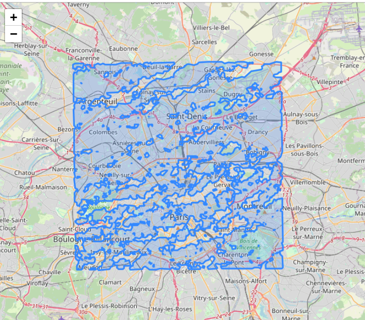
Vector predictions#
We can load the vector output using GeoPandas and then display it over an interactive map using Folium:
[ ]:
%pip install -q folium
[ ]:
from os.path import join
import folium
import numpy as np
import geopandas as gpd

gdf = gpd.read_file(join(out_dir, 'vector_output', 'class-1-cloud.json'))
loc = np.array(gdf.unary_union.centroid.xy).squeeze().tolist()[::-1]
m = folium.Map(location=loc, zoom_start=12)
folium.GeoJson(gdf).add_to(m)
m