The Raster Vision Pipeline#
Raster Vision allows engineers to quickly and repeatably configure pipelines that go through core components of a machine learning workflow: analyzing training data, creating training chips, training models, creating predictions, evaluating models, and bundling the model files and configuration for easy deployment.
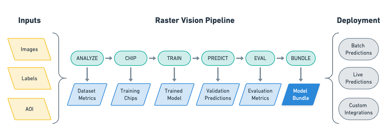
The input to a Raster Vision pipeline is a set of images and training data, optionally with Areas of Interest (AOIs) that describe where the images are labeled. The output of a Raster Vision pipeline is a model bundle that allows you to easily utilize models in various deployment scenarios.
The pipelines include running the following commands:
ANALYZE: Gather dataset-level statistics and metrics for use in downstream processes.
CHIP: Create training chips from a variety of image and label sources.
TRAIN: Train a model using a “backend” such as PyTorch.
PREDICT: Make predictions using trained models on validation and test data.
EVAL: Derive evaluation metrics such as F1 score, precision and recall against the model’s predictions on validation datasets.
BUNDLE: Bundle the trained model and associated configuration into a model bundle, which can be deployed in batch processes, live servers, and other workflows.
Pipelines are configured using a compositional, programmatic approach that makes configuration easy to read, reuse, and maintain. Below, we show the tiny_spacenet example.
from os.path import join
from rastervision.core.rv_pipeline import *
from rastervision.core.backend import *
from rastervision.core.data import *
from rastervision.pytorch_backend import *
from rastervision.pytorch_learner import *


def get_config(runner) -> SemanticSegmentationConfig:
    output_root_uri = '/opt/data/output/tiny_spacenet'
    class_config = ClassConfig(
        names=['building', 'background'], colors=['red', 'black'])

    base_uri = ('https://s3.amazonaws.com/azavea-research-public-data/'
                'raster-vision/examples/spacenet')
    train_image_uri = join(base_uri, 'RGB-PanSharpen_AOI_2_Vegas_img205.tif')
    train_label_uri = join(base_uri, 'buildings_AOI_2_Vegas_img205.geojson')
    val_image_uri = join(base_uri, 'RGB-PanSharpen_AOI_2_Vegas_img25.tif')
    val_label_uri = join(base_uri, 'buildings_AOI_2_Vegas_img25.geojson')

    train_scene = make_scene('scene_205', train_image_uri, train_label_uri,
                             class_config)
    val_scene = make_scene('scene_25', val_image_uri, val_label_uri,
                           class_config)
    scene_dataset = DatasetConfig(
        class_config=class_config,
        train_scenes=[train_scene],
        validation_scenes=[val_scene])

    # Use the PyTorch backend for the SemanticSegmentation pipeline.
    chip_sz = 300

    backend = PyTorchSemanticSegmentationConfig(
        data=SemanticSegmentationGeoDataConfig(
            scene_dataset=scene_dataset,
            sampling=WindowSamplingConfig(
                # randomly sample training chips from scene
                method=WindowSamplingMethod.random,
                # ... of size chip_sz x chip_sz
                size=chip_sz,
                # ... and at most 10 chips per scene
                max_windows=10)),
        model=SemanticSegmentationModelConfig(backbone=Backbone.resnet50),
        solver=SolverConfig(lr=1e-4, num_epochs=1, batch_sz=2))

    return SemanticSegmentationConfig(
        root_uri=output_root_uri,
        dataset=scene_dataset,
        backend=backend,
        predict_options=SemanticSegmentationPredictOptions(chip_sz=chip_sz))


def make_scene(scene_id: str, image_uri: str, label_uri: str,
               class_config: ClassConfig) -> SceneConfig:
    """Define a Scene with image and labels from the given URIs."""

    raster_source = RasterioSourceConfig(
        uris=image_uri,
        # use only the first 3 bands
        channel_order=[0, 1, 2],
    )

    # configure GeoJSON reading
    vector_source = GeoJSONVectorSourceConfig(
        uris=label_uri,
        # The geoms in the label GeoJSON do not have a "class_id" property, so
        # classes must be inferred. Since all geoms are for the building class,
        # this is easy to do: we just assign the building class ID to all of
        # them.
        transformers=[
            ClassInferenceTransformerConfig(
                default_class_id=class_config.get_class_id('building'))
        ])
    # configure transformation of vector data into semantic segmentation labels
    label_source = SemanticSegmentationLabelSourceConfig(
        # semantic segmentation labels must be rasters, so rasterize the geoms
        raster_source=RasterizedSourceConfig(
            vector_source=vector_source,
            rasterizer_config=RasterizerConfig(
                # What about pixels outside of any geoms? Mark them as
                # background.
                background_class_id=class_config.get_class_id('background'))))

    return SceneConfig(
        id=scene_id,
        raster_source=raster_source,
        label_source=label_source,
    )
Raster Vision uses a unittest-like method for executing pipelines. For instance, if the above was defined in tiny_spacenet.py, with the proper setup you could run the experiment on AWS Batch by running:
> rastervision run batch tiny_spacenet.py
See the Quickstart for a more complete description of using this example.