Note
This page was generated from reading_raster_data.ipynb.
Note
If running outside of the Docker image, you may need to set some environment variables manually. You can do it like so:
import os
from subprocess import check_output

os.environ['GDAL_DATA'] = check_output('pip show rasterio | grep Location | awk \'{print $NF"/rasterio/gdal_data/"}\'', shell=True).decode().strip()
We will be accessing files on S3 in this notebook. Since those files are public, we set the AWS_NO_SIGN_REQUEST to tell rasterio to skip the sign-in.
[ ]:
%env AWS_NO_SIGN_REQUEST=YES
Reading raster data#
Reading rasters using RasterSource#
The RasterSource is Raster Vision’s abstraction for windowed reading from a raster image.
One concrete implementation of it is the RasterioSource which is a wrapper around the rasterio library and allows reading from all file formats supported by it.
We can create one from an image like shown below. allow_streaming=True allows us to take advantage of rasterio’s remote-file-reading capabilities; setting it to False will cause Raster Vision to download the image.
[2]:
from rastervision.core.data import RasterioSource

img_uri = 's3://azavea-research-public-data/raster-vision/examples/spacenet/RGB-PanSharpen_AOI_2_Vegas_img205.tif'
raster_source = RasterioSource(img_uri, allow_streaming=True)
[3]:
raster_source.shape
[3]:
(650, 650, 3)
[4]:
raster_source.dtype
[4]:
dtype('uint16')
Reading chips#
RasterSources support numpy-like array slicing, so we can read a smaller chip within the full raster like so:
[5]:
chip = raster_source[:400, :400]
chip.shape
[5]:
(400, 400, 3)
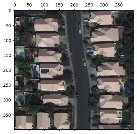
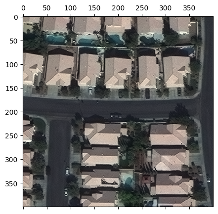
The returned chip is a numpy array which we can plot using matplotlib. Note that since the values are uint16, we first normalize them before plotting.
[6]:
from matplotlib import pyplot as plt

colors_mins = chip.reshape(-1, chip.shape[-1]).min(axis=0)
colors_maxs = chip.reshape(-1, chip.shape[-1]).max(axis=0)
chip_normalized = (chip - colors_mins) / (colors_maxs - colors_mins)

fig, ax = plt.subplots(figsize=(5, 5))
ax.matshow(chip_normalized)
plt.show()
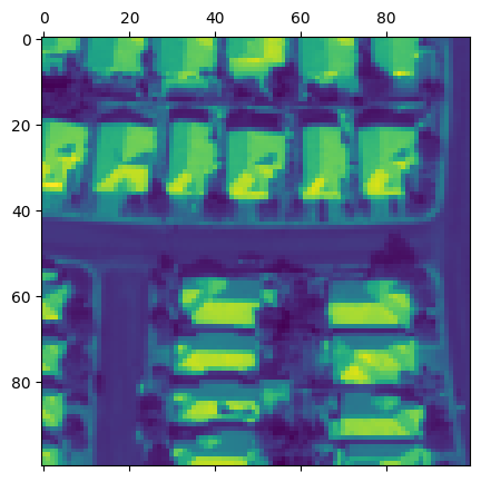
We can even do slightly fancier indexing. The example below reads a 400x400 chip from the the first band in the raster, subsampled to 100x100.
[7]:
chip = raster_source[:400:4, :400:4, [0]]
print('chip.shape:', chip.shape)

fig, ax = plt.subplots(figsize=(5, 5))
ax.matshow(chip)
plt.show()
chip.shape: (100, 100, 1)
The fancy slicing is just syntactic-sugar for the RasterioSource.get_chip() method. The last call is internally translated to the following call to the get_chip() method:
[8]:
from rastervision.core.box import Box

chip = raster_source.get_chip(
    window=Box(ymin=0, xmin=0, ymax=400, xmax=400),
    out_shape=(100, 100),
    bands=[0])
chip.shape
[8]:
(100, 100, 1)
Learn more about the handy Box class here.
Transforming rasters using RasterTransformers#
RasterSources accept a list of RasterTransformers, all of which are automatically applied (in the order specified) to each chip sampled from that RasterSource.
Below we’ll look at two such `RasterTransformer`s:
But Raster Vision also provides the following:
CastTransformer: type-cast chip.NanTransformer: map NaN values to another value.ReclassTransformer: map values to other values using a given mapping; most useful for modifying class IDs in semantic segmentation labels.RGBClassTransformer: if your semantic segmentation labels are in the form of an RGB raster with different colors representing different classes, use this to map them to class IDs.
MinMaxTransformer#
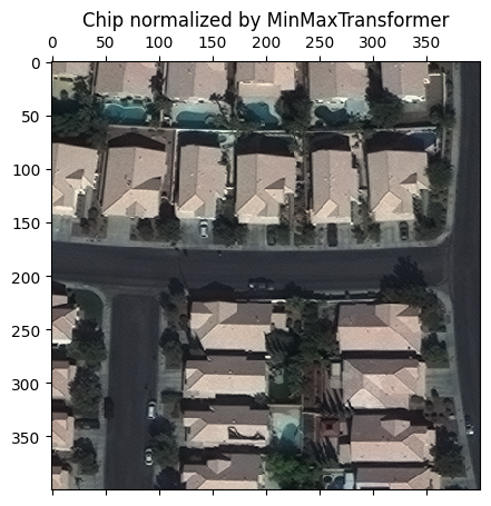
Above, we manually min-max normalized the uint16 chip to 0-1. If we wanted this normalization to be automatically applied to all chips sampled from a RasterSource, we can simply attach a MinMaxTransformer to that RasterSource.
[9]:
from rastervision.core.data import RasterioSource, MinMaxTransformer

img_uri = 's3://azavea-research-public-data/raster-vision/examples/spacenet/RGB-PanSharpen_AOI_2_Vegas_img205.tif'
raster_source = RasterioSource(img_uri, allow_streaming=True)

raster_source_normalized = RasterioSource(
    img_uri,
    allow_streaming=True,
    raster_transformers=[MinMaxTransformer()])
[10]:
from matplotlib import pyplot as plt

chip = raster_source_normalized[:400, :400]

fig, ax = plt.subplots(figsize=(5, 5))
ax.matshow(chip)
ax.set_title('Chip normalized by MinMaxTransformer')
plt.show()
StatsTransformer#
Another useful RasterTransformer is the StatsTransformer.
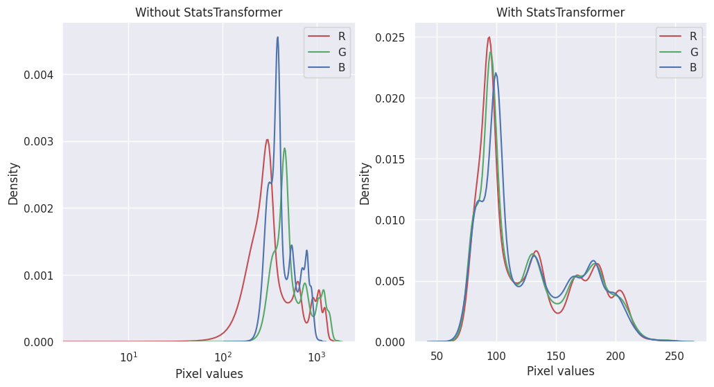
Unlike MinMaxTransformer, the StatsTransformer is able to deal with outlier values. It works by using channel means and standard deviations to convert values to z-scores and then clipping them to some number of standard deviations before scaling to 0-255 and converting to uint8.
We can create and use one like so:
[11]:
from rastervision.core import RasterStats
from rastervision.core.data import RasterioSource, StatsTransformer

img_uri = 's3://azavea-research-public-data/raster-vision/examples/spacenet/RGB-PanSharpen_AOI_2_Vegas_img205.tif'
raster_source = RasterioSource(img_uri, allow_streaming=True)

stats_transformer = StatsTransformer.from_raster_sources(
    raster_sources=[raster_source],
    max_stds=3)

raster_source_normalized = RasterioSource(
    img_uri,
    allow_streaming=True,
    raster_transformers=[stats_transformer])
[12]:
stats_transformer.means, stats_transformer.stds
[12]:
(array([573.68478889, 717.76125556, 516.56731111]),
 array([352.14221914, 350.19743176, 206.5486214 ]))
[13]:
from matplotlib import pyplot as plt

chip_normalized = raster_source_normalized[:400, :400]

fig, ax = plt.subplots(figsize=(5, 5))
ax.matshow(chip_normalized)
ax.set_title('Chip normalized by StatsTransformer')
plt.show()
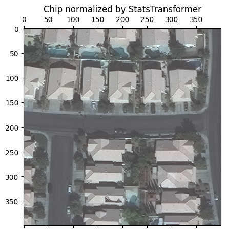
To get a closer look at StatsTransformer’s work, we can visualize each band’s pixel intensity distributions with and without it:
[14]:
import seaborn as sns
sns.reset_defaults()
sns.set_theme()

band_names = 'RGB'

raster_source_unnormalized = RasterioSource(img_uri, allow_streaming=True)
chip_unnormalized = raster_source_unnormalized[:400, :400]

fig, (ax_l, ax_r) = plt.subplots(1, 2, squeeze=True, figsize=(12, 6))

# left
for i in range(chip_unnormalized.shape[-1]):
    sns.kdeplot(chip_unnormalized[..., i].flat, ax=ax_l, c=band_names[i].lower(), label=band_names[i])
ax_l.set_xscale('log')
ax_l.set_xlabel('Pixel values')
ax_l.legend()
ax_l.set_title('Without StatsTransformer')

# right
for i in range(chip_normalized.shape[-1]):
    sns.kdeplot(
        chip_normalized[..., i].flat, ax=ax_r, c=band_names[i].lower(), label=band_names[i])
ax_r.set_xlabel('Pixel values')
ax_r.legend()
ax_r.set_title('With StatsTransformer')

plt.show()
sns.reset_defaults()
Subsetting and reordering bands#
Dealing with multi-band imagery is a commonn use case in the GIS domain. All parts of Raster Vision work seamlessly with arbitrary number of bands.
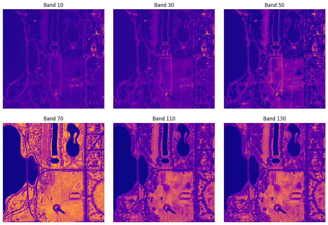
The following example shows how we can use RasterioSource to sample 6 specific channels from a 191-band hyperspectral image.
Data from: https://engineering.purdue.edu/~biehl/MultiSpec/hyperspectral.html
[ ]:
!wget "http://cobweb.ecn.purdue.edu/~biehl/Hyperspectral_Project.zip" -P "data"
!apt install unzip
!unzip "data/Hyperspectral_Project.zip" -d "data/"
There are 2 ways to do this. We can either instantiate a RasterioSource like normal and sample the subset of bands using array indexing…
[25]:
from rastervision.core.data import RasterioSource, MinMaxTransformer

img_uri = 'data/Hyperspectral_Project/dc.tif'
raster_source_hsi = RasterioSource(img_uri)

raster_source_hsi.shape, raster_source_hsi.dtype
Warning 1: TIFFReadDirectory:Sum of Photometric type-related color channels and ExtraSamples doesn't match SamplesPerPixel. Defining non-color channels as ExtraSamples.
[25]:
((1280, 307, 191), dtype('int16'))
[26]:
chip = raster_source_hsi[:100, :100, [10, 30, 50, 70, 110, 130]]
chip.shape
[26]:
(100, 100, 6)
… Or we can specify the channel_order param while instantiating the RasterioSource, which will automatically restrict all sampled chips to these bands.
[27]:
raster_source_hsi = RasterioSource(
    img_uri,
    channel_order=[10, 30, 50, 70, 110, 130],
    raster_transformers=[MinMaxTransformer()])

raster_source_hsi.shape, raster_source_hsi.dtype
Warning 1: TIFFReadDirectory:Sum of Photometric type-related color channels and ExtraSamples doesn't match SamplesPerPixel. Defining non-color channels as ExtraSamples.
[27]:
((1280, 307, 6), dtype('uint8'))
[28]:
chip = raster_source_hsi[200:500, :]
chip.shape
[28]:
(300, 307, 6)
[48]:
fig, axs = plt.subplots(2, 3, squeeze=True, figsize=(12, 8))
fig.tight_layout(h_pad=1.5, w_pad=-1)
for i, (ax, ch) in enumerate(zip(axs.flat, raster_source_hsi.channel_order)):
    ax.matshow(chip[..., i], cmap='plasma')
    ax.set_title(f'Band {ch}')
    ax.set_xticks([], [])
    ax.set_yticks([], [])
    ax.axis('off')
plt.show()
Combining bands from different files using MultiRasterSource#
Another common use case is combining bands from multiple sources. This can done using a MultiRasterSource.
The following example combines RGB, SWIR, and SAR bands into a single 8-band RasterSource.
Data from: Cloud to Street - Microsoft flood dataset
[49]:
uri_seninel_2_rgb = 'https://radiantearth.blob.core.windows.net/mlhub/c2smsfloods/chips/e7d1917e-c069-45cf-a392-42e24aa2f4ac/s2/S2A_MSIL1C_20201022T100051_N0209_R122_T33UXP_20201022T111023_07680-00512/RGB.png'
uri_seninel_2_swir = 'https://radiantearth.blob.core.windows.net/mlhub/c2smsfloods/chips/e7d1917e-c069-45cf-a392-42e24aa2f4ac/s2/S2A_MSIL1C_20201022T100051_N0209_R122_T33UXP_20201022T111023_07680-00512/SWIR.png'
uri_seninel_1_vh = 'https://radiantearth.blob.core.windows.net/mlhub/c2smsfloods/chips/e7d1917e-c069-45cf-a392-42e24aa2f4ac/s1/S1B_IW_GRDH_1SDV_20201020T164222_20201020T164247_023899_02D6C4_35D8_07680-00512/VH.tif'
uri_seninel_1_vv = 'https://radiantearth.blob.core.windows.net/mlhub/c2smsfloods/chips/e7d1917e-c069-45cf-a392-42e24aa2f4ac/s1/S1B_IW_GRDH_1SDV_20201020T164222_20201020T164247_023899_02D6C4_35D8_07680-00512/VV.tif'
First, we create RasterSources for each individual source.
[50]:
from rastervision.core.data import RasterioSource, MultiRasterSource, MinMaxTransformer

rs_sentinel_2_rgb = RasterioSource(uri_seninel_2_rgb, allow_streaming=True)
rs_sentinel_2_swir = RasterioSource(uri_seninel_2_swir, allow_streaming=True)

rs_seninel_1_vh = RasterioSource(uri_seninel_1_vh, allow_streaming=True, raster_transformers=[MinMaxTransformer()])
rs_seninel_1_vv = RasterioSource(uri_seninel_1_vv, allow_streaming=True, raster_transformers=[MinMaxTransformer()])

print('rs_sentinel_2_rgb', rs_sentinel_2_rgb.shape, rs_sentinel_2_rgb.dtype)
print('rs_sentinel_2_swir', rs_sentinel_2_swir.shape, rs_sentinel_2_swir.dtype)
print('rs_seninel_1_vh', rs_seninel_1_vh.shape, rs_seninel_1_vh.dtype)
print('rs_seninel_1_vv', rs_seninel_1_vv.shape, rs_seninel_1_vv.dtype)
rs_sentinel_2_rgb (512, 512, 3) uint8
rs_sentinel_2_swir (512, 512, 3) uint8
rs_seninel_1_vh (512, 512, 1) uint8
rs_seninel_1_vv (512, 512, 1) uint8
Next, we combine them into a MultiRasterSource.
[51]:
raster_sources = [
    rs_sentinel_2_rgb,
    rs_sentinel_2_swir,
    rs_seninel_1_vh,
    rs_seninel_1_vv
]

raster_source_multi = MultiRasterSource(
    raster_sources=raster_sources, primary_source_idx=0)

raster_source_multi.shape, raster_source_multi.dtype
[51]:
((512, 512, 8), dtype('uint8'))
[52]:
chip = raster_source_multi[:, :]
chip.shape
[52]:
(512, 512, 8)
[61]:
from matplotlib import pyplot as plt

fig, (ax_rgb, ax_swir, ax_vh, ax_vv) = plt.subplots(1, 4, figsize=(15, 4))

ax_rgb.matshow(chip[..., :3])
ax_rgb.set_title('RGB')
ax_swir.matshow(chip[..., 3:6])
ax_swir.set_title('SWIR')
ax_vh.matshow(chip[..., 6])
ax_vh.set_title('VH')
ax_vv.matshow(chip[..., 7])
ax_vv.set_title('VV')

plt.show()

Creating a time-series of images using TemporalMultiRasterSource#
Let’s pretend that rs_seninel_1_vh and rs_seninel_1_vh are images of the same area from two different times. Then we can stack them into a time-series as below.
[62]:
from rastervision.core.data import TemporalMultiRasterSource

raster_sources = [
    rs_seninel_1_vh,
    rs_seninel_1_vv
]
raster_source_temporal = TemporalMultiRasterSource(raster_sources=raster_sources)
raster_source_temporal.shape
[62]:
(2, 512, 512, 1)
See also the notebook:Working with time-series of images
Cropping the extent#
Sometimes you might want to crop a RasterSource. For example, if you want to use one part of it for training and another for validation. You can do this via the bbox param.
The following example shows how we can crop out the top 200 pixels and left 200 pixels of the full raster.
[63]:
from rastervision.core.data import RasterioSource, MinMaxTransformer
from rastervision.core.box import Box

img_uri = 's3://azavea-research-public-data/raster-vision/examples/spacenet/RGB-PanSharpen_AOI_2_Vegas_img205.tif'
raster_source_cropped = RasterioSource(
    img_uri,
    allow_streaming=True,
    bbox=Box(200, 200, 650, 650),
    raster_transformers=[MinMaxTransformer()])

raster_source_cropped.shape, raster_source_cropped.dtype
[63]:
((450, 450, 3), dtype('uint8'))
[66]:
from rastervision.core.box import Box
from matplotlib import pyplot as plt

chip = raster_source_cropped[:400, :400]
print(chip.shape)

fig, ax = plt.subplots(figsize=(5, 5))
ax.matshow(chip)
plt.show()
(400, 400, 3)
